Discover superior methods for hyperparameter optimization with Amazon SageMaker Computerized Mannequin Tuning
Creating high-performance machine studying (ML) options depends on exploring and optimizing coaching parameters, often known as hyperparameters. Hyperparameters are the knobs and levers that we use to regulate the coaching course of, resembling studying charge, batch measurement, regularization energy, and others, relying on the particular mannequin and job at hand. Exploring hyperparameters entails systematically various the values of every parameter and observing the impression on mannequin efficiency. Though this course of requires further efforts, the advantages are vital. Hyperparameter optimization (HPO) can result in quicker coaching occasions, improved mannequin accuracy, and higher generalization to new knowledge.
We proceed our journey from the publish Optimize hyperparameters with Amazon SageMaker Automatic Model Tuning. We beforehand explored a single job optimization, visualized the outcomes for SageMaker built-in algorithm, and discovered concerning the impression of specific hyperparameter values. On prime of utilizing HPO as a one-time optimization on the finish of the mannequin creation cycle, we will additionally use it throughout a number of steps in a conversational method. Every tuning job helps us get nearer to efficiency, however moreover, we additionally learn the way delicate the mannequin is to sure hyperparameters and might use this understanding to tell the following tuning job. We are able to revise the hyperparameters and their worth ranges primarily based on what we discovered and subsequently flip this optimization effort right into a dialog. And in the identical means that we as ML practitioners accumulate data over these runs, Amazon SageMaker Automatic Model Tuning (AMT) with heat begins can preserve this data acquired in earlier tuning jobs for the following tuning job as nicely.
On this publish, we run a number of HPO jobs with a {custom} coaching algorithm and completely different HPO methods resembling Bayesian optimization and random search. We additionally put heat begins into motion and visually evaluate our trials to refine hyperparameter area exploration.
Superior ideas of SageMaker AMT
Within the subsequent sections, we take a more in-depth take a look at every of the next subjects and present how SageMaker AMT may also help you implement them in your ML initiatives:
- Use {custom} coaching code and the favored ML framework Scikit-learn in SageMaker Coaching
- Outline {custom} analysis metrics primarily based on the logs for analysis and optimization
- Carry out HPO utilizing an applicable technique
- Use heat begins to show a single hyperparameter search right into a dialog with our mannequin
- Use superior visualization methods utilizing our answer library to match two HPO methods and tuning jobs outcomes
Whether or not you’re utilizing the built-in algorithms utilized in our first publish or your personal coaching code, SageMaker AMT gives a seamless person expertise for optimizing ML fashions. It supplies key performance that lets you deal with the ML drawback at hand whereas robotically holding monitor of the trials and outcomes. On the identical time, it robotically manages the underlying infrastructure for you.
On this publish, we transfer away from a SageMaker built-in algorithm and use {custom} code. We use a Random Forest from SkLearn. However we persist with the identical ML job and dataset as in our first post, which is detecting handwritten digits. We cowl the content material of the Jupyter pocket book 2_advanced_tuning_with_custom_training_and_visualizing.ipynb and invite you to invoke the code aspect by aspect to learn additional.
Let’s dive deeper and uncover how we will use {custom} coaching code, deploy it, and run it, whereas exploring the hyperparameter search area to optimize our outcomes.
The right way to construct an ML mannequin and carry out hyperparameter optimization
What does a typical course of for constructing an ML answer appear like? Though there are lots of potential use circumstances and a big number of ML duties on the market, we propose the next psychological mannequin for a stepwise method:
- Perceive your ML state of affairs at hand and choose an algorithm primarily based on the necessities. For instance, you may wish to remedy a picture recognition job utilizing a supervised studying algorithm. On this publish, we proceed to make use of the handwritten picture recognition state of affairs and the identical dataset as in our first publish.
- Resolve which implementation of the algorithm in SageMaker Coaching you wish to use. There are numerous choices, inside SageMaker or exterior ones. Moreover, it’s good to outline which underlying metric suits finest in your job and also you wish to optimize for (resembling accuracy, F1 rating, or ROC). SageMaker helps 4 choices relying in your wants and assets:
- Use a pre-trained mannequin through Amazon SageMaker JumpStart, which you need to use out of the field or simply fine-tune it.
- Use one of many built-in algorithms for coaching and tuning, like XGBoost, as we did in our earlier publish.
- Practice and tune a {custom} mannequin primarily based on one of many main frameworks like Scikit-learn, TensorFlow, or PyTorch. AWS supplies a choice of pre-made Docker pictures for this function. For this publish, we use this feature, which lets you experiment rapidly by operating your personal code on prime of a pre-made container picture.
- Convey your personal {custom} Docker picture in case you wish to use a framework or software program that isn’t in any other case supported. This selection requires essentially the most effort, but additionally supplies the best diploma of flexibility and management.
- Practice the mannequin together with your knowledge. Relying on the algorithm implementation from the earlier step, this may be so simple as referencing your coaching knowledge and operating the coaching job or by moreover offering {custom} code for coaching. In our case, we use some {custom} coaching code in Python primarily based on Scikit-learn.
- Apply hyperparameter optimization (as a “dialog” together with your ML mannequin). After the coaching, you sometimes wish to optimize the efficiency of your mannequin by discovering essentially the most promising mixture of values in your algorithm’s hyperparameters.
Relying in your ML algorithm and mannequin measurement, the final step of hyperparameter optimization might grow to be an even bigger problem than anticipated. The next questions are typical for ML practitioners at this stage and may sound acquainted to you:
- What sort of hyperparameters are impactful for my ML drawback?
- How can I successfully search an enormous hyperparameter area to search out these best-performing values?
- How does the mix of sure hyperparameter values affect my efficiency metric?
- Prices matter; how can I exploit my assets in an environment friendly method?
- What sort of tuning experiments are worthwhile, and the way can I evaluate them?
It’s not simple to reply these questions, however there’s excellent news. SageMaker AMT takes the heavy lifting from you, and allows you to consider choosing the proper HPO technique and worth ranges you wish to discover. Moreover, our visualization answer facilitates the iterative evaluation and experimentation course of to effectively discover well-performing hyperparameter values.
Within the subsequent sections, we construct a digit recognition mannequin from scratch utilizing Scikit-learn and present all these ideas in motion.
Resolution overview
SageMaker gives some very useful options to coach, consider, and tune our mannequin. It covers all performance of an end-to-end ML lifecycle, so we don’t even want to go away our Jupyter pocket book.
In our first publish, we used the SageMaker built-in algorithm XGBoost. For demonstration functions, this time we swap to a Random Forest classifier as a result of we will then present learn how to present your personal coaching code. We opted for offering our personal Python script and utilizing Scikit-learn as our framework. Now, how will we specific that we wish to use a selected ML framework? As we’ll see, SageMaker makes use of one other AWS service within the background to retrieve a pre-built Docker container picture for coaching—Amazon Elastic Container Registry (Amazon ECR).
We cowl the next steps intimately, together with code snippets and diagrams to attach the dots. As talked about earlier than, you probably have the possibility, open the pocket book and run the code cells step-by-step to create the artifacts in your AWS atmosphere. There isn’t any higher means of lively studying.
- First, load and put together the information. We use Amazon Simple Storage Service (Amazon S3) to add a file containing our handwritten digits knowledge.
- Subsequent, put together the coaching script and framework dependencies. We offer the {custom} coaching code in Python, reference some dependent libraries, and make a take a look at run.
- To outline the {custom} goal metrics, SageMaker lets us outline a daily expression to extract the metrics we want from the container log recordsdata.
- Practice the mannequin utilizing the scikit-learn framework. By referencing a pre-built container picture, we create a corresponding Estimator object and go our {custom} coaching script.
- AMT permits us to check out numerous HPO methods. We consider two of them for this publish: random search and Bayesian search.
- Select between SageMaker HPO methods.
- Visualize, analyze, and evaluate tuning outcomes. Our visualization package deal permits us to find which technique performs higher and which hyperparameter values ship the most effective efficiency primarily based on our metrics.
- Proceed the exploration of the hyperparameter area and heat begin HPO jobs.
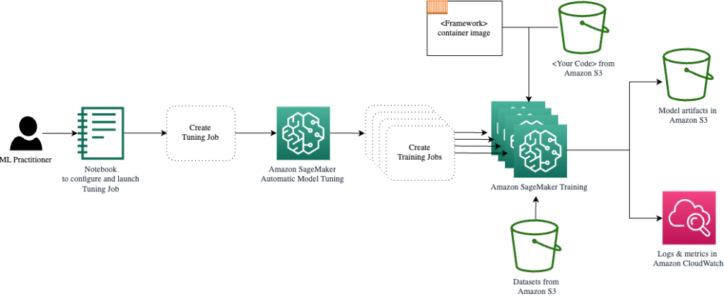
AMT takes care of scaling and managing the underlying compute infrastructure to run the assorted tuning jobs on Amazon Elastic Compute Cloud (Amazon EC2) situations. This manner, you don’t have to burden your self to provision situations, deal with any working system and {hardware} points, or mixture log recordsdata by yourself. The ML framework picture is retrieved from Amazon ECR and the mannequin artifacts together with tuning outcomes are saved in Amazon S3. All logs and metrics are collected in Amazon CloudWatch for handy entry and additional evaluation if wanted.
Conditions
As a result of it is a continuation of a sequence, it is suggested, however not essentially required, to learn our first post about SageMaker AMT and HPO. Other than that, fundamental familiarity with ML ideas and Python programming is useful. We additionally suggest following together with every step within the accompanying notebook from our GitHub repository whereas studying this publish. The pocket book may be run independently from the primary one, however wants some code from subfolders. Be sure that to clone the complete repository in your atmosphere as described within the README file.
Experimenting with the code and utilizing the interactive visualization choices vastly enhances your studying expertise. So, please test it out.
Load and put together the information
As a primary step, we ensure that the downloaded digits data we want for coaching is accessible to SageMaker. Amazon S3 permits us to do that in a secure and scalable means. Check with the pocket book for the whole supply code and be at liberty to adapt it with your personal knowledge.
The digits.csv file accommodates function knowledge and labels. Every digit is represented by pixel values in an 8×8 picture, as depicted by the next picture for the digit 4.
Put together the coaching script and framework dependencies
Now that the information is saved in our S3 bucket, we will outline our {custom} coaching script primarily based on Scikit-learn in Python. SageMaker provides us the choice to easily reference the Python file later for coaching. Any dependencies just like the Scikit-learn or pandas libraries may be supplied in two methods:
- They are often specified explicitly in a
necessities.txtfile - They’re pre-installed within the underlying ML container picture, which is both supplied by SageMaker or custom-built
Each choices are typically thought-about normal methods for dependency administration, so that you may already be aware of it. SageMaker helps a variety of ML frameworks in a ready-to-use managed atmosphere. This consists of most of the hottest knowledge science and ML frameworks like PyTorch, TensorFlow, or Scikit-learn, as in our case. We don’t use an extra necessities.txt file, however be at liberty so as to add some libraries to strive it out.
The code of our implementation accommodates a technique known as match(), which creates a brand new classifier for the digit recognition job and trains it. In distinction to our first publish the place we used the SageMaker built-in XGBoost algorithm, we now use a RandomForestClassifier supplied by the ML library sklearn. The decision of the match() technique on the classifier object begins the coaching course of utilizing a subset (80%) of our CSV knowledge:
See the complete script in our Jupyter pocket book on GitHub.
Earlier than you spin up container assets for the complete coaching course of, did you attempt to run the script immediately? It is a good apply to rapidly make sure the code has no syntax errors, verify for matching dimensions of your knowledge buildings, and another errors early on.
There are two methods to run your code domestically. First, you may run it straight away within the pocket book, which additionally lets you use the Python Debugger pdb:
Alternatively, run the prepare script from the command line in the identical means chances are you’ll wish to use it in a container. This additionally helps setting numerous parameters and overwriting the default values as wanted, for instance:
As output, you may see the primary outcomes for the mannequin’s efficiency primarily based on the target metrics precision, recall, and F1-score. For instance, pre: 0.970 rec: 0.969 f1: 0.969.
Not unhealthy for such a fast coaching. However the place did these numbers come from and what will we do with them?
Outline {custom} goal metrics
Keep in mind, our purpose is to totally prepare and tune our mannequin primarily based on the target metrics we take into account related for our job. As a result of we use a {custom} coaching script, we have to outline these metrics for SageMaker explicitly.
Our script emits the metrics precision, recall, and F1-score throughout coaching just by utilizing the print operate:
The usual output is captured by SageMaker and despatched to CloudWatch as a log stream. To retrieve the metric values and work with them later in SageMaker AMT, we have to present some info on learn how to parse that output. We are able to obtain this by defining common expression statements (for extra info, seek advice from Monitor and Analyze Training Jobs Using Amazon CloudWatch Metrics):
Let’s stroll via the primary metric definition within the previous code collectively. SageMaker will search for output within the log that begins with pre: and is adopted by a number of whitespace after which a quantity that we wish to extract, which is why we use the spherical parenthesis. Each time SageMaker finds a worth like that, it turns it right into a CloudWatch metric with the title valid-precision.
Practice the mannequin utilizing the Scikit-learn framework
After we create our coaching script prepare.py and instruct SageMaker on learn how to monitor the metrics inside CloudWatch, we outline a SageMaker Estimator object. It initiates the coaching job and makes use of the occasion sort we specify. However how can this occasion sort be completely different from the one you run an Amazon SageMaker Studio pocket book on, and why? SageMaker Studio runs your coaching (and inference) jobs on separate compute situations than your pocket book. This lets you proceed working in your pocket book whereas the roles run within the background.
The parameter framework_version refers back to the Scikit-learn model we use for our coaching job. Alternatively, we will go image_uri to the estimator. You possibly can verify whether or not your favourite framework or ML library is accessible as a pre-built SageMaker Docker image and use it as is or with extensions.
Furthermore, we will run SageMaker coaching jobs on EC2 Spot Cases by setting use_spot_instances to True. They’re spare capability situations that may save up to 90% of costs. These situations present flexibility on when the coaching jobs are run.
After the Estimator object is ready up, we begin the coaching by calling the match() operate, supplying the trail to the coaching dataset on Amazon S3. We are able to use this identical technique to offer validation and take a look at knowledge. We set the wait parameter to True so we will use the educated mannequin within the subsequent code cells.
estimator.match({'prepare': s3_data_url}, wait=True)Outline hyperparameters and run tuning jobs
Thus far, we’ve got educated the mannequin with one set of hyperparameter values. However had been these values good? Or may we search for higher ones? Let’s use the HyperparameterTuner class to run a scientific search over the hyperparameter area. How will we search this area with the tuner? The mandatory parameters are the target metric title and goal sort that can information the optimization. The optimization technique is one other key argument for the tuner as a result of it additional defines the search area. The next are 4 completely different methods to select from:
- Grid search
- Random search
- Bayesian optimization (default)
- Hyperband
We additional describe these methods and equip you with some steerage to decide on one later on this publish.
Earlier than we outline and run our tuner object, let’s recap our understanding from an structure perspective. We lined the architectural overview of SageMaker AMT in our last post and reproduce an excerpt of it right here for comfort.

We are able to select what hyperparameters we wish to tune or depart static. For dynamic hyperparameters, we offer hyperparameter_ranges that can be utilized to optimize for tunable hyperparameters. As a result of we use a Random Forest classifier, we’ve got utilized the hyperparameters from the Scikit-learn Random Forest documentation.
We additionally restrict assets with the utmost variety of coaching jobs and parallel coaching jobs the tuner can use. We are going to see how these limits assist us evaluate the outcomes of assorted methods with one another.
Much like the Estimator’s match operate, we begin a tuning job calling the tuner’s match:
That is all we’ve got to do to let SageMaker run the coaching jobs (n=50) within the background, every utilizing a unique set of hyperparameters. We discover the outcomes later on this publish. However earlier than that, let’s begin one other tuning job, this time making use of the Bayesian optimization technique. We are going to evaluate each methods visually after their completion.
Notice that each tuner jobs can run in parallel as a result of SageMaker orchestrates the required compute situations independently of one another. That’s fairly useful for practitioners who experiment with completely different approaches on the identical time, like we do right here.
Select between SageMaker HPO methods
In the case of tuning methods, you may have a couple of choices with SageMaker AMT: grid search, random search, Bayesian optimization, and Hyperband. These methods decide how the automated tuning algorithms discover the required ranges of hyperparameters.
Random search is fairly easy. It randomly selects combos of values from the required ranges and may be run in a sequential or parallel method. It’s like throwing darts blindfolded, hoping to hit the goal. We have now began with this technique, however will the outcomes enhance with one other one?
Bayesian optimization takes a unique method than random search. It considers the historical past of earlier choices and chooses values which are more likely to yield the most effective outcomes. If you wish to be taught from earlier explorations, you may obtain this solely with operating a brand new tuning job after the earlier ones. Is sensible, proper? On this means, Bayesian optimization depends on the earlier runs. However do you see what HPO technique permits for increased parallelization?
Hyperband is an fascinating one! It makes use of a multi-fidelity technique, which implies it dynamically allocates assets to essentially the most promising coaching jobs and stops these which are underperforming. Due to this fact, Hyperband is computationally environment friendly with assets, studying from earlier coaching jobs. After stopping the underperforming configurations, a brand new configuration begins, and its values are chosen randomly.
Relying in your wants and the character of your mannequin, you may select between random search, Bayesian optimization, or Hyperband as your tuning technique. Every has its personal method and benefits, so it’s vital to think about which one works finest in your ML exploration. The excellent news for ML practitioners is which you can choose the most effective HPO technique by visually evaluating the impression of every trial on the target metric. Within the subsequent part, we see learn how to visually determine the impression of various methods.
Visualize, analyze, and evaluate tuning outcomes
When our tuning jobs are full, it will get thrilling. What outcomes do they ship? What sort of increase are you able to count on on our metric in comparison with your base mannequin? What are the best-performing hyperparameters for our use case?
A fast and simple solution to view the HPO outcomes is by visiting the SageMaker console. Below Hyperparameter tuning jobs, we will see (per tuning job) the mix of hyperparameter values which have been examined and delivered the most effective efficiency as measured by our goal metric (valid-f1).

Is that every one you want? As an ML practitioner, chances are you’ll be not solely thinking about these values, however definitely wish to be taught extra concerning the internal workings of your mannequin to discover its full potential and strengthen your instinct with empirical suggestions.
visualization device can vastly enable you perceive the development by HPO over time and get empirical suggestions on design choices of your ML mannequin. It exhibits the impression of every particular person hyperparameter in your goal metric and supplies steerage to additional optimize your tuning outcomes.
We use the amtviz {custom} visualization package deal to visualise and analyze tuning jobs. It’s easy to make use of and supplies useful options. We reveal its profit by decoding some particular person charts, and at last evaluating random search aspect by aspect with Bayesian optimization.
First, let’s create a visualization for random search. We are able to do that by calling visualize_tuning_job() from amtviz and passing our first tuner object as an argument:
You will note a few charts, however let’s take it step-by-step. The primary scatter plot from the output seems like the next and already provides us some visible clues we wouldn’t acknowledge in any desk.

Every dot represents the efficiency of a person coaching job (our goal valid-f1 on the y-axis) primarily based on its begin time (x-axis), produced by a selected set of hyperparameters. Due to this fact, we take a look at the efficiency of our mannequin because it progresses over the period of the tuning job.
The dotted line highlights the most effective end result discovered to this point and signifies enchancment over time. The most effective two coaching jobs achieved an F1 rating of round 0.91.
Apart from the dotted line displaying the cumulative progress, do you see a pattern within the chart?
In all probability not. And that is anticipated, as a result of we’re viewing the outcomes of the random HPO technique. Every coaching job was run utilizing a unique however randomly chosen set of hyperparameters. If we continued our tuning job (or ran one other one with the identical setting), we might most likely see some higher outcomes over time, however we will’t make certain. Randomness is a difficult factor.
The following charts enable you gauge the affect of hyperparameters on the general efficiency. All hyperparameters are visualized, however for the sake of brevity, we deal with two of them: n-estimators and max-depth.

Our prime two coaching jobs had been utilizing n-estimators of round 20 and 80, and max-depth of round 10 and 18, respectively. The precise hyperparameter values are displayed through tooltip for every dot (coaching job). They’re even dynamically highlighted throughout all charts and provide you with a multi-dimensional view! Did you see that? Every hyperparameter is plotted in opposition to the target metric, as a separate chart.
Now, what sort of insights will we get about n-estimators?
Primarily based on the left chart, evidently very low worth ranges (under 10) extra typically ship poor outcomes in comparison with increased values. Due to this fact, increased values might assist your mannequin to carry out higher—fascinating.
In distinction, the correlation of the max-depth hyperparameter to our goal metric is somewhat low. We are able to’t clearly inform which worth ranges are performing higher from a basic perspective.
In abstract, random search may also help you discover a well-performing set of hyperparameters even in a comparatively quick period of time. Additionally, it isn’t biased in direction of answer however provides a balanced view of the search area. Your useful resource utilization, nevertheless, won’t be very environment friendly. It continues to run coaching jobs with hyperparameters in worth ranges which are recognized to ship poor outcomes.
Let’s look at the outcomes of our second tuning job utilizing Bayesian optimization. We are able to use amtviz to visualise the leads to the identical means as we did to this point for the random search tuner. Or, even higher, we will use the aptitude of the operate to match each tuning jobs in a single set of charts. Fairly useful!

There are extra dots now as a result of we visualize the outcomes of all coaching jobs for each, the random search (orange dots) and the Bayesian optimization (blue dots). On the best aspect, you may see a density chart visualizing the distribution of all F1-scores. A majority of the coaching jobs achieved leads to the higher a part of the F1 scale (over 0.6)—that’s good!
What’s the key takeaway right here? The scatter plot clearly exhibits the good thing about Bayesian optimization. It delivers higher outcomes over time as a result of it could actually be taught from earlier runs. That’s why we achieved considerably higher outcomes utilizing Bayesian in comparison with random (0.967 vs. 0.919) with the identical variety of coaching jobs.
There may be much more you are able to do with amtviz. Let’s drill in.
If you happen to give SageMaker AMT the instruction to run a bigger variety of jobs for tuning, seeing many trials directly can get messy. That’s one of many explanation why we made these charts interactive. You possibly can click on and drag on each hyperparameter scatter plot to zoom in to sure worth ranges and refine your visible interpretation of the outcomes. All different charts are robotically up to date. That’s fairly useful, isn’t it? See the following charts for instance and check out it for your self in your pocket book!

As a tuning maximalist, you may additionally determine that operating one other hyperparameter tuning job may additional enhance your mannequin efficiency. However this time, a extra particular vary of hyperparameter values may be explored since you already know (roughly) the place to count on higher outcomes. For instance, chances are you’ll select to deal with values between 100–200 for n-estimators, as proven within the chart. This lets AMT deal with essentially the most promising coaching jobs and will increase your tuning effectivity.
To sum it up, amtviz supplies you with a wealthy set of visualization capabilities that assist you to higher perceive the impression of your mannequin’s hyperparameters on efficiency and allow smarter choices in your tuning actions.
Proceed the exploration of the hyperparameter area and heat begin HPO jobs
We have now seen that AMT helps us discover the hyperparameter search area effectively. However what if we want a number of rounds of tuning to iteratively enhance our outcomes? As talked about at first, we wish to set up an optimization suggestions cycle—our “dialog” with the mannequin. Do we have to begin from scratch each time?
Let’s look into the idea of operating a warm start hyperparameter tuning job. It doesn’t provoke new tuning jobs from scratch, it reuses what has been discovered within the earlier HPO runs. This helps us be extra environment friendly with our tuning time and compute assets. We are able to additional iterate on prime of our earlier outcomes. To make use of heat begins, we create a WarmStartConfig and specify warm_start_type as IDENTICAL_DATA_AND_ALGORITHM. Because of this we modify the hyperparameter values however we don’t change the information or algorithm. We inform AMT to switch the earlier data to our new tuning job.
By referring to our earlier Bayesian optimization and random search tuning jobs as mother and father, we will use them each for the nice and cozy begin:
To see the good thing about utilizing heat begins, seek advice from the next charts. These are generated by amtviz in an identical means as we did earlier, however this time we’ve got added one other tuning job primarily based on a heat begin.

Within the left chart, we will observe that new tuning jobs principally lie within the upper-right nook of the efficiency metric graph (see dots marked in orange). The nice and cozy begin has certainly reused the earlier outcomes, which is why these knowledge factors are within the prime outcomes for F1 rating. This enchancment can be mirrored within the density chart on the best.
In different phrases, AMT robotically selects promising units of hyperparameter values primarily based on its data from earlier trials. That is proven within the subsequent chart. For instance, the algorithm would take a look at a low worth for n-estimators much less actually because these are recognized to provide poor F1 scores. We don’t waste any assets on that, due to heat begins.

Clear up
To keep away from incurring undesirable prices while you’re executed experimenting with HPO, you need to take away all recordsdata in your S3 bucket with the prefix amt-visualize-demo and in addition shut down SageMaker Studio resources.
Run the next code in your pocket book to take away all S3 recordsdata from this publish:
If you happen to want to maintain the datasets or the mannequin artifacts, chances are you’ll modify the prefix within the code to amt-visualize-demo/knowledge to solely delete the information or amt-visualize-demo/output to solely delete the mannequin artifacts.
Conclusion
We have now discovered how the artwork of constructing ML options entails exploring and optimizing hyperparameters. Adjusting these knobs and levers is a demanding but rewarding course of that results in quicker coaching occasions, improved mannequin accuracy, and total higher ML options. The SageMaker AMT performance helps us run a number of tuning jobs and heat begin them, and supplies knowledge factors for additional assessment, visible comparability, and evaluation.
On this publish, we regarded into HPO methods that we use with SageMaker AMT. We began with random search, a simple however performant technique the place hyperparameters are randomly sampled from a search area. Subsequent, we in contrast the outcomes to Bayesian optimization, which makes use of probabilistic fashions to information the seek for optimum hyperparameters. After we recognized an acceptable HPO technique and good hyperparameter worth ranges via preliminary trials, we confirmed learn how to use heat begins to streamline future HPO jobs.
You possibly can discover the hyperparameter search area by evaluating quantitative outcomes. We have now advised the side-by-side visible comparability and supplied the mandatory package deal for interactive exploration. Tell us within the feedback how useful it was for you in your hyperparameter tuning journey!
In regards to the authors
 Ümit Yoldas is a Senior Options Architect with Amazon Net Companies. He works with enterprise clients throughout industries in Germany. He’s pushed to translate AI ideas into real-world options. Exterior of labor, he enjoys time with household, savoring good meals, and pursuing health.
 Elina Lesyk is a Options Architect positioned in Munich. She is specializing in enterprise clients from the monetary companies business. In her free time, you’ll find Elina constructing purposes with generative AI at some IT meetups, driving a brand new thought on fixing local weather change quick, or operating within the forest to organize for a half-marathon with a typical deviation from the deliberate schedule.
 Mariano Kamp is a Principal Options Architect with Amazon Net Companies. He works with banks and insurance coverage firms in Germany on machine studying. In his spare time, Mariano enjoys climbing along with his spouse.


