Differentially non-public median and extra – Google Analysis Weblog

Differential privacy (DP) is a rigorous mathematical definition of privateness. DP algorithms are randomized to guard person knowledge by guaranteeing that the likelihood of any specific output is almost unchanged when an information level is added or eliminated. Subsequently, the output of a DP algorithm doesn’t disclose the presence of anybody knowledge level. There was vital progress in each foundational analysis and adoption of differential privateness with contributions such because the Privacy Sandbox and Google Open Source Library.

ML and knowledge analytics algorithms can usually be described as performing a number of primary computation steps on the identical dataset. When every such step is differentially non-public, so is the output, however with a number of steps the general privateness assure deteriorates, a phenomenon referred to as the value of composition. Composition theorems sure the rise in privateness loss with the quantity okay of computations: Within the normal case, the privateness loss will increase with the sq. root of okay. Because of this we want a lot stricter privateness ensures for every step with the intention to meet our total privateness assure objective. However in that case, we lose utility. A technique to enhance the privateness vs. utility trade-off is to establish when the use circumstances admit a tighter privateness evaluation than what follows from composition theorems.

Good candidates for such enchancment are when every step is utilized to a disjoint half (slice) of the dataset. When the slices are chosen in a data-independent method, every level impacts solely one of many okay outputs and the privateness ensures don’t deteriorate with okay. Nevertheless, there are functions wherein we have to choose the slices adaptively (that’s, in a method that will depend on the output of prior steps). In these circumstances, a change of a single knowledge level could cascade — altering a number of slices and thus rising composition value.

In “Õptimal Differentially Private Learning of Thresholds and Quasi-Concave Optimization”, introduced at STOC 2023, we describe a brand new paradigm that enables for slices to be chosen adaptively and but avoids composition value. We present that DP algorithms for a number of basic aggregation and studying duties may be expressed on this Reorder-Slice-Compute (RSC) paradigm, gaining vital enhancements in utility.

The Reorder-Slice-Compute (RSC) paradigm

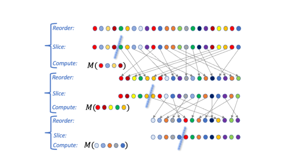
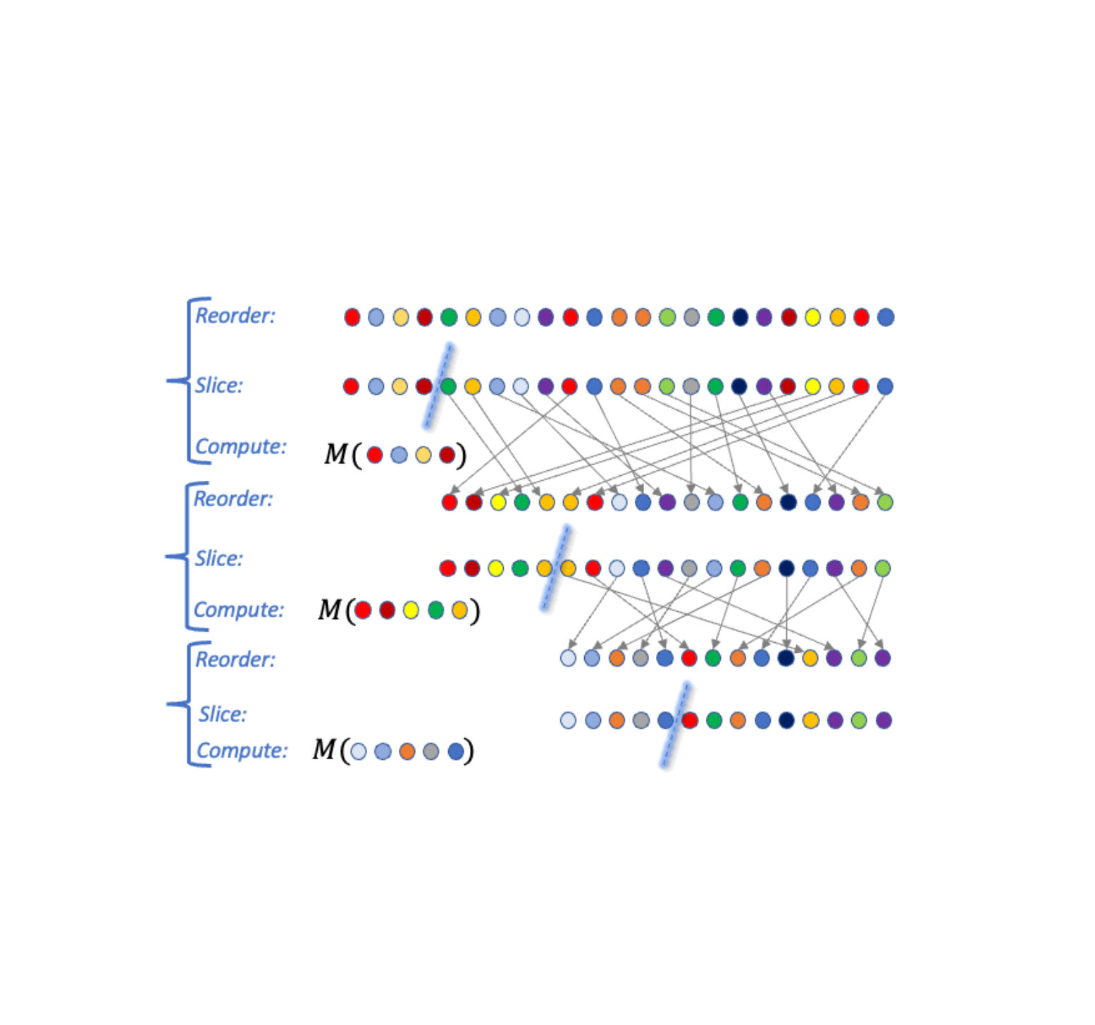
An algorithm A falls within the RSC paradigm if it may be expressed within the following normal kind (see visualization under). The enter is a delicate set D of knowledge factors. The algorithm then performs a sequence of okay steps as follows:

1. Choose an ordering over knowledge factors, a slice dimension m, and a DP algorithm M. The choice could rely on the output of A in prior steps (and therefore is adaptive).
2. Slice out the (roughly) high m knowledge factors in accordance with the order from the dataset D, apply M to the slice, and output the end result.

A visualization of three Reorder-Slice-Compute (RSC) steps.

If we analyze the general privateness lack of an RSC algorithm utilizing DP composition theorems, the privateness assure suffers from the anticipated composition value, i.e., it deteriorates with the sq. root of the variety of steps okay. To remove this composition value, we offer a novel evaluation that removes the dependence on okay altogether: the general privateness assure is near that of a single step! The concept behind our tighter evaluation is a novel approach that limits the potential cascade of affected steps when a single knowledge level is modified (particulars in the paper).

Tighter privateness evaluation means higher utility. The effectiveness of DP algorithms is usually said when it comes to the smallest enter dimension (variety of knowledge factors) that suffices with the intention to launch an accurate end result that meets the privateness necessities. We describe a number of issues with algorithms that may be expressed within the RSC paradigm and for which our tighter evaluation improved utility.

Non-public interval level

We begin with the next primary aggregation job. The enter is a dataset D of n factors from an ordered area X (consider the area because the pure numbers between 1 and |X|). The objective is to return a degree y in X that’s within the interval of D, that’s between the minimal and the utmost factors in D.

The answer to the interval level drawback is trivial with out the privateness requirement: merely return any level within the dataset D. However this resolution isn’t privacy-preserving because it discloses the presence of a selected datapoint within the enter. We are able to additionally see that if there is just one level within the dataset, a privacy-preserving resolution isn’t attainable, because it should return that time. We are able to due to this fact ask the next basic query: What’s the smallest enter dimension N for which we will clear up the non-public interval level drawback?

It’s identified that N should improve with the area dimension |X| and that this dependence is not less than the iterated log function log* |X| [1, 2]. However, the best prior DP algorithm required the enter dimension to be not less than (log* |X|)^1.5. To shut this hole, we designed an RSC algorithm that requires solely an order of log* |X| factors.

The iterated log function is extraordinarily gradual rising: It’s the variety of instances we have to take a logarithm of a price earlier than we attain a price that is the same as or smaller than 1. How did this operate naturally come out within the evaluation? Every step of the RSC algorithm remapped the area to a logarithm of its prior dimension. Subsequently there have been log* |X| steps in complete. The tighter RSC evaluation eradicated a sq. root of the variety of steps from the required enter dimension.

Though the interval level job appears very primary, it captures the essence of the issue of personal options for frequent aggregation duties. We subsequent describe two of those duties and specific the required enter dimension to those duties when it comes to N.

Non-public approximate median

One among these frequent aggregation duties is approximate median: The enter is a dataset D of n factors from an ordered area X. The objective is to return a degree y that’s between the ⅓ and ⅔ quantiles of D. That’s, not less than a 3rd of the factors in D are smaller or equal to y and not less than a 3rd of the factors are bigger or equal to y. Be aware that returning an actual median isn’t attainable with differential privateness, because it discloses the presence of a datapoint. Therefore we take into account the relaxed requirement of an approximate median (proven under).

We are able to compute an approximate median by discovering an interval level: We slice out the N smallest factors and the N largest factors after which compute an interval level of the remaining factors. The latter should be an approximate median. This works when the dataset dimension is not less than 3N.

An instance of an information D over area X, the set of interval factors, and the set of approximate medians.

Non-public studying of axis-aligned rectangles

For the subsequent job, the enter is a set of n labeled knowledge factors, the place every level x = (x₁,….,x_d) is a d-dimensional vector over a site X. Displayed under, the objective is to be taught values a_i , b_i for the axes i=1,…,d that outline a d-dimensional rectangle, in order that for every instance x

• If x is positively labeled (proven as crimson plus indicators under) then it lies throughout the rectangle, that’s, for all axes i, x_i is within the interval [a_i ,b_i], and
• If x is negatively labeled (proven as blue minus indicators under) then it lies outdoors the rectangle, that’s, for not less than one axis i, x_i is outdoors the interval [a_i ,b_i].

A set of 2-dimensional labeled factors and a respective rectangle.

Any DP resolution for this drawback should be approximate in that the realized rectangle should be allowed to mislabel some knowledge factors, with some positively labeled factors outdoors the rectangle or negatively labeled factors inside it. It’s because an actual resolution could possibly be very delicate to the presence of a selected knowledge level and wouldn’t be non-public. The objective is a DP resolution that retains this essential variety of mislabeled factors small.

We first take into account the one-dimensional case (d = 1). We’re on the lookout for an interval [a,b] that covers all optimistic factors and not one of the unfavorable factors. We present that we will do that with at most 2N mislabeled factors. We deal with the positively labeled factors. Within the first RSC step we slice out the N smallest factors and compute a personal interval level as a. We then slice out the N largest factors and compute a personal interval level as b. The answer [a,b] appropriately labels all negatively labeled factors and mislabels at most 2N of the positively labeled factors. Thus, at most ~2N factors are mislabeled in complete.

Illustration for d = 1, we slice out N left optimistic factors and compute an interval level a, slice out N proper optimistic factors and compute an interval level b.

With d > 1, we iterate over the axes i = 1,….,d and apply the above for the i^th coordinates of enter factors to acquire the values a_i , b_i . In every iteration, we carry out two RSC steps and slice out 2N positively labeled factors. In complete, we slice out 2dN factors and all remaining factors have been appropriately labeled. That’s, all negatively-labeled factors are outdoors the ultimate d-dimensional rectangle and all positively-labeled factors, besides maybe ~2dN, lie contained in the rectangle. Be aware that this algorithm makes use of the complete flexibility of RSC in that the factors are ordered in another way by every axis. Since we carry out d steps, the RSC evaluation shaves off an element of sq. root of d from the variety of mislabeled factors.

Coaching ML fashions with adaptive choice of coaching examples

The coaching effectivity or efficiency of ML fashions can typically be improved by choosing coaching examples in a method that will depend on the present state of the mannequin, e.g., self-paced curriculum learning or active learning.

The most typical methodology for personal coaching of ML fashions is DP-SGD, the place noise is added to the gradient replace from every minibatch of coaching examples. Privateness evaluation with DP-SGD usually assumes that coaching examples are randomly partitioned into minibatches. But when we impose a data-dependent choice order on coaching examples, and additional modify the choice standards okay instances throughout coaching, then evaluation by way of DP composition leads to deterioration of the privateness ensures of a magnitude equal to the sq. root of okay.

Thankfully, instance choice with DP-SGD may be naturally expressed within the RSC paradigm: every choice standards reorders the coaching examples and every minibatch is a slice (for which we compute a loud gradient). With RSC evaluation, there isn’t a privateness deterioration with okay, which brings DP-SGD coaching with instance choice into the sensible area.

Conclusion

The RSC paradigm was launched with the intention to sort out an open drawback that’s primarily of theoretical significance, however seems to be a flexible instrument with the potential to reinforce knowledge effectivity in manufacturing environments.

Acknowledgments

The work described right here was achieved collectively with Xin Lyu, Jelani Nelson, and Tamas Sarlos.