Classifying Duplicate Questions from Quora with Keras

Introduction

On this put up we’ll use Keras to categorise duplicated questions from Quora.
The dataset first appeared within the Kaggle competitors Quora Question Pairs and consists of roughly 400,000 pairs of questions together with a column indicating if the query pair is taken into account a reproduction.

Our implementation is impressed by the Siamese Recurrent Architecture, with modifications to the similarity
measure and the embedding layers (the unique paper makes use of pre-trained phrase vectors). Utilizing this type
of structure dates again to 2005 with Le Cun et al and is beneficial for
verification duties. The concept is to be taught a perform that maps enter patterns right into a
goal house such {that a} similarity measure within the goal house approximates
the “semantic” distance within the enter house.

After the competitors, Quora additionally described their strategy to this downside on this blog post.

Dowloading information

Knowledge could be downloaded from the Kaggle dataset webpage
or from Quora’s release of the dataset:

library(keras)
quora_data <- get_file(
  "quora_duplicate_questions.tsv",
  "https://qim.ec.quoracdn.internet/quora_duplicate_questions.tsv"
)

We’re utilizing the Keras get_file() perform in order that the file obtain is cached.

Studying and preprocessing

We’ll first load information into R and do some preprocessing to make it simpler to
embrace within the mannequin. After downloading the information, you may learn it
utilizing the readr read_tsv() perform.

We’ll create a Keras tokenizer to rework every phrase into an integer
token. We may even specify a hyperparameter of our mannequin: the vocabulary measurement.
For now let’s use the 50,000 commonest phrases (we’ll tune this parameter later).
The tokenizer will likely be match utilizing all distinctive questions from the dataset.

tokenizer <- text_tokenizer(num_words = 50000)
tokenizer %>% fit_text_tokenizer(unique(c(df$question1, df$question2)))

Let’s save the tokenizer to disk to be able to use it for inference later.

save_text_tokenizer(tokenizer, "tokenizer-question-pairs")

We’ll now use the textual content tokenizer to rework every query into a listing
of integers.

question1 <- texts_to_sequences(tokenizer, df$question1)
question2 <- texts_to_sequences(tokenizer, df$question2)

Let’s check out the variety of phrases in every query. This can helps us to
determine the padding size, one other hyperparameter of our mannequin. Padding the sequences normalizes them to the identical measurement in order that we are able to feed them to the Keras mannequin.

80% 90% 95% 99% 
 14  18  23  31 

We will see that 99% of questions have at most size 31 so we’ll select a padding
size between 15 and 30. Let’s begin with 20 (we’ll additionally tune this parameter later).
The default padding worth is 0, however we’re already utilizing this worth for phrases that
don’t seem inside the 50,000 most frequent, so we’ll use 50,001 as a substitute.

question1_padded <- pad_sequences(question1, maxlen = 20, worth = 50000 + 1)
question2_padded <- pad_sequences(question2, maxlen = 20, worth = 50000 + 1)

Now we have now completed the preprocessing steps. We’ll now run a easy benchmark
mannequin earlier than transferring on to the Keras mannequin.

Easy benchmark

Earlier than creating a sophisticated mannequin let’s take a easy strategy.
Let’s create two predictors: share of phrases from question1 that
seem within the question2 and vice-versa. Then we’ll use a logistic
regression to foretell if the questions are duplicate.

perc_words_question1 <- map2_dbl(question1, question2, ~mean(.x %in% .y))
perc_words_question2 <- map2_dbl(question2, question1, ~mean(.x %in% .y))

df_model <- data.frame(
  perc_words_question1 = perc_words_question1,
  perc_words_question2 = perc_words_question2,
  is_duplicate = df$is_duplicate
) %>%
  na.omit()

Now that now we have our predictors, let’s create the logistic mannequin.
We’ll take a small pattern for validation.

val_sample <- sample.int(nrow(df_model), 0.1*nrow(df_model))
logistic_regression <- glm(
  is_duplicate ~ perc_words_question1 + perc_words_question2, 
  household = "binomial",
  information = df_model[-val_sample,]
)
summary(logistic_regression)

Name:
glm(formulation = is_duplicate ~ perc_words_question1 + perc_words_question2, 
    household = "binomial", information = df_model[-val_sample, ])

Deviance Residuals: 
    Min       1Q   Median       3Q      Max  
-1.5938  -0.9097  -0.6106   1.1452   2.0292  

Coefficients:
                      Estimate Std. Error z worth Pr(>|z|)    
(Intercept)          -2.259007   0.009668 -233.66   <2e-16 ***
perc_words_question1  1.517990   0.023038   65.89   <2e-16 ***
perc_words_question2  1.681410   0.022795   73.76   <2e-16 ***
---
Signif. codes:  0 ‘***’ 0.001 ‘**’ 0.01 ‘*’ 0.05 ‘.’ 0.1 ‘ ’ 1

(Dispersion parameter for binomial household taken to be 1)

    Null deviance: 479158  on 363843  levels of freedom
Residual deviance: 431627  on 363841  levels of freedom
  (17 observations deleted as a consequence of missingness)
AIC: 431633

Variety of Fisher Scoring iterations: 3

Let’s calculate the accuracy on our validation set.

pred <- predict(logistic_regression, df_model[val_sample,], sort = "response")
pred <- pred > mean(df_model$is_duplicate[-val_sample])
accuracy <- table(pred, df_model$is_duplicate[val_sample]) %>% 
  prop.table() %>% 
  diag() %>% 
  sum()
accuracy

[1] 0.6573577

We bought an accuracy of 65.7%. Not all that a lot better than random guessing.
Now let’s create our mannequin in Keras.

Mannequin definition

We’ll use a Siamese community to foretell whether or not the pairs are duplicated or not.
The concept is to create a mannequin that may embed the questions (sequence of phrases)
right into a vector. Then we are able to evaluate the vectors for every query utilizing a similarity
measure and inform if the questions are duplicated or not.

First let’s outline the inputs for the mannequin.

input1 <- layer_input(form = c(20), title = "input_question1")
input2 <- layer_input(form = c(20), title = "input_question2")

Then let’s the outline the a part of the mannequin that can embed the questions in a
vector.

word_embedder <- layer_embedding( 
  input_dim = 50000 + 2, # vocab measurement + UNK token + padding worth
  output_dim = 128,      # hyperparameter - embedding measurement
  input_length = 20,     # padding measurement,
  embeddings_regularizer = regularizer_l2(0.0001) # hyperparameter - regularization 
)

seq_embedder <- layer_lstm(
  models = 128, # hyperparameter -- sequence embedding measurement
  kernel_regularizer = regularizer_l2(0.0001) # hyperparameter - regularization 
)

Now we’ll outline the connection between the enter vectors and the embeddings
layers. Word that we use the identical layers and weights on each inputs. That’s why
that is referred to as a Siamese community. It is sensible, as a result of we don’t need to have totally different
outputs if question1 is switched with question2.

vector1 <- input1 %>% word_embedder() %>% seq_embedder()
vector2 <- input2 %>% word_embedder() %>% seq_embedder()

We then outline the similarity measure we need to optimize. We wish duplicated questions
to have larger values of similarity. On this instance we’ll use the cosine similarity,
however any similarity measure might be used. Keep in mind that the cosine similarity is the
normalized dot product of the vectors, however for coaching it’s not essential to
normalize the outcomes.

cosine_similarity <- layer_dot(list(vector1, vector2), axes = 1)

Subsequent, we outline a closing sigmoid layer to output the chance of each questions
being duplicated.

output <- cosine_similarity %>% 
  layer_dense(models = 1, activation = "sigmoid")

Now that permit’s outline the Keras mannequin when it comes to it’s inputs and outputs and
compile it. Within the compilation part we outline our loss perform and optimizer.
Like within the Kaggle problem, we’ll decrease the logloss (equal
to minimizing the binary crossentropy). We’ll use the Adam optimizer.

mannequin <- keras_model(list(input1, input2), output)
mannequin %>% compile(
  optimizer = "adam", 
  metrics = list(acc = metric_binary_accuracy), 
  loss = "binary_crossentropy"
)

We will then check out out mannequin with the abstract perform.

_______________________________________________________________________________________
Layer (sort)                Output Form       Param #    Linked to                 
=======================================================================================
input_question1 (InputLayer (None, 20)         0                                       
_______________________________________________________________________________________
input_question2 (InputLayer (None, 20)         0                                       
_______________________________________________________________________________________
embedding_1 (Embedding)     (None, 20, 128)    6400256    input_question1[0][0]        
                                                          input_question2[0][0]        
_______________________________________________________________________________________
lstm_1 (LSTM)               (None, 128)        131584     embedding_1[0][0]            
                                                          embedding_1[1][0]            
_______________________________________________________________________________________
dot_1 (Dot)                 (None, 1)          0          lstm_1[0][0]                 
                                                          lstm_1[1][0]                 
_______________________________________________________________________________________
dense_1 (Dense)             (None, 1)          2          dot_1[0][0]                  
=======================================================================================
Whole params: 6,531,842
Trainable params: 6,531,842
Non-trainable params: 0
_______________________________________________________________________________________

Mannequin becoming

Now we’ll match and tune our mannequin. Nonetheless earlier than continuing let’s take a pattern for validation.

set.seed(1817328)
val_sample <- sample.int(nrow(question1_padded), measurement = 0.1*nrow(question1_padded))

train_question1_padded <- question1_padded[-val_sample,]
train_question2_padded <- question2_padded[-val_sample,]
train_is_duplicate <- df$is_duplicate[-val_sample]

val_question1_padded <- question1_padded[val_sample,]
val_question2_padded <- question2_padded[val_sample,]
val_is_duplicate <- df$is_duplicate[val_sample]

Now we use the match() perform to coach the mannequin:

mannequin %>% match(
  list(train_question1_padded, train_question2_padded),
  train_is_duplicate, 
  batch_size = 64, 
  epochs = 10, 
  validation_data = list(
    list(val_question1_padded, val_question2_padded), 
    val_is_duplicate
  )
)

Practice on 363861 samples, validate on 40429 samples
Epoch 1/10
363861/363861 [==============================] - 89s 245us/step - loss: 0.5860 - acc: 0.7248 - val_loss: 0.5590 - val_acc: 0.7449
Epoch 2/10
363861/363861 [==============================] - 88s 243us/step - loss: 0.5528 - acc: 0.7461 - val_loss: 0.5472 - val_acc: 0.7510
Epoch 3/10
363861/363861 [==============================] - 88s 242us/step - loss: 0.5428 - acc: 0.7536 - val_loss: 0.5439 - val_acc: 0.7515
Epoch 4/10
363861/363861 [==============================] - 88s 242us/step - loss: 0.5353 - acc: 0.7595 - val_loss: 0.5358 - val_acc: 0.7590
Epoch 5/10
363861/363861 [==============================] - 88s 242us/step - loss: 0.5299 - acc: 0.7633 - val_loss: 0.5358 - val_acc: 0.7592
Epoch 6/10
363861/363861 [==============================] - 88s 242us/step - loss: 0.5256 - acc: 0.7662 - val_loss: 0.5309 - val_acc: 0.7631
Epoch 7/10
363861/363861 [==============================] - 88s 242us/step - loss: 0.5211 - acc: 0.7701 - val_loss: 0.5349 - val_acc: 0.7586
Epoch 8/10
363861/363861 [==============================] - 88s 242us/step - loss: 0.5173 - acc: 0.7733 - val_loss: 0.5278 - val_acc: 0.7667
Epoch 9/10
363861/363861 [==============================] - 88s 242us/step - loss: 0.5138 - acc: 0.7762 - val_loss: 0.5292 - val_acc: 0.7667
Epoch 10/10
363861/363861 [==============================] - 88s 242us/step - loss: 0.5092 - acc: 0.7794 - val_loss: 0.5313 - val_acc: 0.7654

After coaching completes, we are able to save our mannequin for inference with the save_model_hdf5()
perform.

save_model_hdf5(mannequin, "model-question-pairs.hdf5")

Mannequin tuning

Now that now we have an inexpensive mannequin, let’s tune the hyperparameters utilizing the
tfruns package deal. We’ll start by including FLAGS declarations to our script for all hyperparameters we need to tune (FLAGS enable us to range hyperparmaeters with out altering our supply code):

FLAGS <- flags(
  flag_integer("vocab_size", 50000),
  flag_integer("max_len_padding", 20),
  flag_integer("embedding_size", 256),
  flag_numeric("regularization", 0.0001),
  flag_integer("seq_embedding_size", 512)
)

With this FLAGS definition we are able to now write our code when it comes to the flags. For instance:

input1 <- layer_input(form = c(FLAGS$max_len_padding))
input2 <- layer_input(form = c(FLAGS$max_len_padding))

embedding <- layer_embedding(
  input_dim = FLAGS$vocab_size + 2, 
  output_dim = FLAGS$embedding_size, 
  input_length = FLAGS$max_len_padding, 
  embeddings_regularizer = regularizer_l2(l = FLAGS$regularization)
)

The total supply code of the script with FLAGS could be discovered here.

We moreover added an early stopping callback within the coaching step to be able to cease coaching
if validation loss doesn’t lower for five epochs in a row. This can hopefully cut back coaching time for unhealthy fashions. We additionally added a studying fee reducer to scale back the educational fee by an element of 10 when the loss doesn’t lower for 3 epochs (this method sometimes will increase mannequin accuracy).

mannequin %>% match(
  ...,
  callbacks = list(
    callback_early_stopping(persistence = 5),
    callback_reduce_lr_on_plateau(persistence = 3)
  )
)

We will now execute a tuning run to probe for the optimum mixture of hyperparameters. We name the tuning_run() perform, passing a listing with
the doable values for every flag. The tuning_run() perform will likely be liable for executing the script for all mixtures of hyperparameters. We additionally specify
the pattern parameter to coach the mannequin for less than a random pattern from all mixtures (decreasing coaching time considerably).

library(tfruns)

runs <- tuning_run(
  "question-pairs.R", 
  flags = list(
    vocab_size = c(30000, 40000, 50000, 60000),
    max_len_padding = c(15, 20, 25),
    embedding_size = c(64, 128, 256),
    regularization = c(0.00001, 0.0001, 0.001),
    seq_embedding_size = c(128, 256, 512)
  ), 
  runs_dir = "tuning", 
  pattern = 0.2
)

The tuning run will return a information.body with outcomes for all runs.
We discovered that one of the best run attained 84.9% accuracy utilizing the mix of hyperparameters proven beneath, so we modify our coaching script to make use of these values because the defaults:

FLAGS <- flags(
  flag_integer("vocab_size", 50000),
  flag_integer("max_len_padding", 20),
  flag_integer("embedding_size", 256),
  flag_numeric("regularization", 1e-4),
  flag_integer("seq_embedding_size", 512)
)

Making predictions

Now that now we have skilled and tuned our mannequin we are able to begin making predictions.
At prediction time we’ll load each the textual content tokenizer and the mannequin we saved
to disk earlier.

library(keras)
mannequin <- load_model_hdf5("model-question-pairs.hdf5", compile = FALSE)
tokenizer <- load_text_tokenizer("tokenizer-question-pairs")

Since we received’t proceed coaching the mannequin, we specified the compile = FALSE argument.

Now let`s outline a perform to create predictions. On this perform we we preprocess the enter information in the identical method we preprocessed the coaching information:

predict_question_pairs <- perform(mannequin, tokenizer, q1, q2) {
  q1 <- texts_to_sequences(tokenizer, list(q1))
  q2 <- texts_to_sequences(tokenizer, list(q2))
  
  q1 <- pad_sequences(q1, 20)
  q2 <- pad_sequences(q2, 20)
  
  as.numeric(predict(mannequin, list(q1, q2)))
}

We will now name it with new pairs of questions, for instance:

predict_question_pairs(
  mannequin,
  tokenizer,
  "What's R programming?",
  "What's R in programming?"
)

[1] 0.9784008

Prediction is kind of quick (~40 milliseconds).

Deploying the mannequin

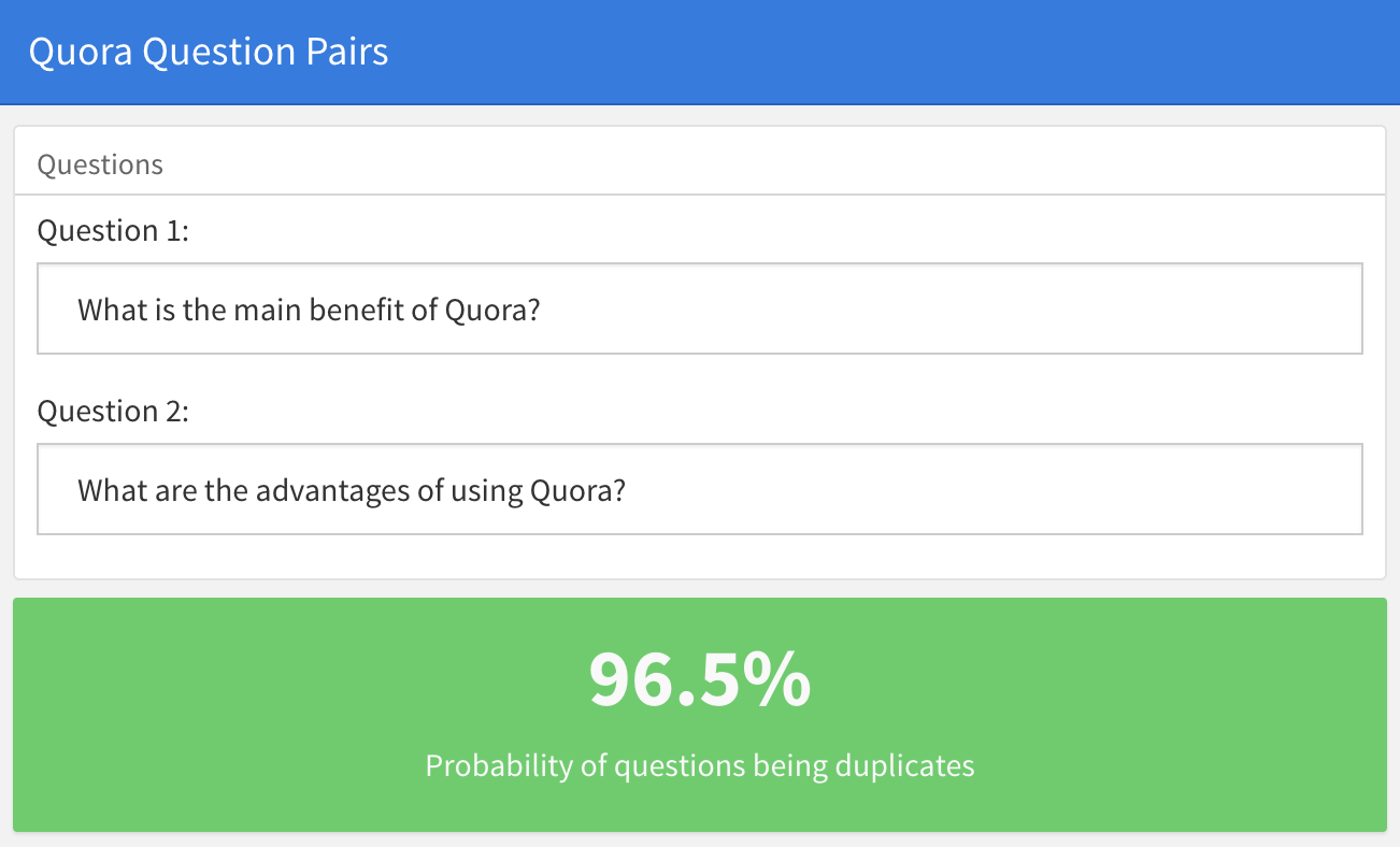
To show deployment of the skilled mannequin, we created a easy Shiny utility, the place
you may paste 2 questions from Quora and discover the chance of them being duplicated. Strive altering the questions beneath or coming into two completely totally different questions.

The shiny utility could be discovered at https://jjallaire.shinyapps.io/shiny-quora/ and it’s supply code at https://github.com/dfalbel/shiny-quora-question-pairs.

Word that when deploying a Keras mannequin you solely have to load the beforehand saved mannequin file and tokenizer (no coaching information or mannequin coaching steps are required).

Wrapping up

• We skilled a Siamese LSTM that provides us cheap accuracy (84%). Quora’s state-of-the-art is 87%.
• We will enhance our mannequin by utilizing pre-trained phrase embeddings on bigger datasets. For instance, attempt utilizing what’s described in this example. Quora makes use of their very own full corpus to coach the phrase embeddings.
• After coaching we deployed our mannequin as a Shiny utility which given two Quora questions calculates the chance of their being duplicates.