Deep Studying for Most cancers Immunotherapy

Introduction

In my analysis, I apply deep studying to unravel molecular interactions within the human immune system. One software of my analysis is inside most cancers immunotherapy (Immuno-oncology or Immunooncology) – a most cancers therapy technique, the place the goal is to make the most of the most cancers affected person’s personal immune system to combat the most cancers.

The goal of this submit is to illustrates how deep studying is efficiently being utilized to mannequin key molecular interactions within the human immune system. Molecular interactions are extremely context dependent and due to this fact non-linear. Deep studying is a robust software to seize non-linearity and has due to this fact confirmed invaluable and extremely profitable. Particularly in modelling the molecular interplay between the Main Histocompability Advanced sort I (MHCI) and peptides (The state-of-the-art mannequin netMHCpan identifies 96.5% of pure peptides at a really excessive specificity of 98.5%).

Adoptive T-cell remedy

Some transient background earlier than diving in. Particular immune cells (T-cells) patrol our physique, scanning the cells to examine if they’re wholesome. On the floor of our cells is the MHCI – a extremely specialised molecular system, which displays the well being standing inside our cells. That is accomplished by displaying small fragments of proteins referred to as peptides, thus reflecting the within of the cell. T-cells probe these molecular shows to examine if the peptides are from our personal physique (self) or international (non-self), e.g. from a virus an infection or most cancers. If a displayed peptide is non-self, the T-cells has the facility to terminate the cell.

Simon Caulton, Adoptive T-cell therapy, CC BY-SA 3.0

Adoptive T-cell remedy is a type of most cancers immunotherapy that goals to isolate tumor infiltrating T-cells from the tumor within the affected person, probably genetically engineer them to be cancer-specific, develop them in nice numbers and reintroduce them into the physique to combat the most cancers. With a purpose to terminate most cancers cells, the T-cell must be activated by being uncovered to tumor peptides certain to MHCI (pMHCI). By analyzing the tumor genetics, related peptides might be recognized and relying on the sufferers explicit sort of MHCI, we will predict which pMHCI are more likely to be current within the tumor within the affected person and thus which pMHCIs needs to be used to activate the T-cells.

Peptide Classification Mannequin

For this use case, we utilized three fashions to categorise whether or not a given peptide is a ‘robust binder’ SB, ‘weak binder’ WB or ‘non-binder’ NB. to MHCI (Particular sort: HLA-A*02:01). Thereby, the classification uncovers which peptides, might be offered to the T-cells. The fashions we examined had been:

• A deep feed ahead absolutely linked ANN
• A convolutional ANN (linked to a FFN)
• A random forest (for comparability)

Subsequent, we’ll dive into constructing the substitute neural community. If you wish to a extra detailed rationalization of most cancers immunotherapy and the way it interacts with the human immune system earlier than going additional, see the primer on cancer immunotherapy on the finish of the submit.

Stipulations

This instance makes use of the keras bundle, a number of tidyverse packages, in addition to the ggseqlogo and PepTools packages. You may set up these packages as follows:

# Keras + TensorFlow and it is dependencies
install.packages("keras")
library(keras)
install_keras()

# Tidyverse (readr, ggplot2, and so forth.)
install.packages("tidyverse")

# Packages for sequence logos and peptides
devtools::install_github("omarwagih/ggseqlogo")
devtools::install_github("leonjessen/PepTools")

We are able to now load all the packages we want for this instance:

Peptide Information

The enter knowledge for this use case was created by producing 1,000,000 random 9-mer peptides by sampling the one-letter code for the 20 amino acids, i.e. ARNDCQEGHILKMFPSTWYV, after which submitting the peptides to MHCI binding prediction utilizing the present state-of-the-art mannequin netMHCpan. Totally different variants of MHCI exists, so for this case we selected HLA-A*02:01. This methodology assigns ‘robust binder’ SB, ‘weak binder’ WB or ‘non-binder’ NB to every peptide.

Since n(SB) < n(WB) << n(NB), the info was subsequently balanced by down sampling, such that n(SB) = n(WB) = n(NB) = 7,920. Thus, a data set with a total of 23,760 data points was created. 10% of the info factors had been randomly assigned as check knowledge and the rest as prepare knowledge. It needs to be famous that because the knowledge set originates from a mannequin, the result of this explicit use case might be a mannequin of a mannequin. Nonetheless, netMHCpan could be very correct (96.5% of pure ligands are recognized at a really excessive specificity 98.5%).

Within the following every peptide might be encoded by assigning a vector of 20 values, the place every worth is the likelihood of the amino acid mutating into 1 of the 20 others as outlined by the BLOSUM62 matrix utilizing the pep_encode() operate from the PepTools bundle. This fashion every peptide is transformed to an ‘picture’ matrix with 9 rows and 20 columns.

Let’s load the info:

pep_file <- get_file(
  "ran_peps_netMHCpan40_predicted_A0201_reduced_cleaned_balanced.tsv", 
  origin = "https://git.io/vb3Xa"
) 
pep_dat <- read_tsv(file = pep_file)

The instance peptide knowledge appears to be like like this:

# A tibble: 5 x 4
  peptide   label_chr label_num data_type
  <chr>     <chr>         <int> <chr>    
1 LLTDAQRIV WB                1 prepare    
2 LMAFYLYEV SB                2 prepare    
3 VMSPITLPT WB                1 check     
4 SLHLTNCFV WB                1 prepare    
5 RQFTCMIAV WB                1 prepare   

The place peptide is the 9-mer peptides, label_chr defines whether or not the peptide was predicted by netMHCpan to be a strong-binder SB, weak-binder WB or NB non-binder to HLA-A*02:01.

label_num is equal to label_chr, such that NB = 0, WB = 1 and SB = 2. Lastly data_type defines whether or not the actual knowledge level is a part of the prepare set used to construct the mannequin or the ~10% knowledge unnoticed check set, which might be used for ultimate efficiency analysis.

The info has been balanced, as proven on this abstract:

pep_dat %>% group_by(label_chr, data_type) %>% summarise(n = n())

# A tibble: 6 x 3
# Teams:   label_chr [?]
  label_chr data_type     n
  <chr>     <chr>     <int>
1 NB        check        782
2 NB        prepare      7138
3 SB        check        802
4 SB        prepare      7118
5 WB        check        792
6 WB        prepare      7128

We are able to use the ggseqlogo bundle to visualise the sequence motif for the robust binders utilizing a sequence brand. This enables us to see which positions within the peptide and which amino acids are crucial for the binding to MHC (Greater letters point out extra significance):

pep_dat %>% filter(label_chr=='SB') %>% pull(peptide) %>% ggseqlogo()

From the sequence brand, it’s evident, that L,M,I,V are discovered typically at p2 and p9 amongst the robust binders. In reality these place are known as the anchor positions, which work together with the MHCI. The T-cell however, will acknowledge p3-p8.

Information Preparation

We’re making a mannequin f, the place x is the peptide and y is considered one of three lessons SB, WB and NB, such that f(x) = y. Every x is encoded right into a 2-dimensional ‘picture’, which we will visualize utilizing the pep_plot_images() operate:

pep_dat %>% filter(label_chr=='SB') %>% head(1) %>% pull(peptide) %>% pep_plot_images

To feed knowledge right into a neural community we have to encode it as a multi-dimensional array (or “tensor”). For this dataset we will do that with the PepTools::pep_encode() operate, which takes a personality vector of peptides and transforms them right into a 3D array of ‘complete variety of peptides’ x ‘size of every peptide (9)’ x ‘variety of distinctive amino acids (20)’. For instance:

str(pep_encode(c("LLTDAQRIV", "LLTDAQRIV")))

 num [1:2, 1:9, 1:20] 0.0445 0.0445 0.0445 0.0445 0.073 ...

Right here’s how we rework the info body into 3-D arrays of coaching and check knowledge:

x_train <- pep_dat %>% filter(data_type == 'prepare') %>% pull(peptide)   %>% pep_encode
y_train <- pep_dat %>% filter(data_type == 'prepare') %>% pull(label_num) %>% array
x_test  <- pep_dat %>% filter(data_type == 'check')  %>% pull(peptide)   %>% pep_encode
y_test  <- pep_dat %>% filter(data_type == 'check')  %>% pull(label_num) %>% array

To organize the info for coaching we convert the 3-D arrays into matrices by reshaping width and top right into a single dimension (9×20 peptide ‘photos’ are flattened into vectors of lengths 180):

x_train <- array_reshape(x_train, c(nrow(x_train), 9, 20, 1))
x_test  <- array_reshape(x_test, c(nrow(x_test), 9, 20, 1))

The y knowledge is an integer vector with values starting from 0 to 2. To organize this knowledge for coaching we one-hot encode the vectors into binary class matrices utilizing the Keras to_categorical operate:

y_train <- to_categorical(y_train, num_classes = 3)
y_test  <- to_categorical(y_test,  num_classes = 3)

Defining the Mannequin

The core knowledge construction of Keras is a mannequin, a method to set up layers. The only sort of mannequin is the sequential mannequin, a linear stack of layers. We start by making a sequential mannequin after which including layers utilizing the pipe (%>%) operator:

mannequin <- keras_model_sequential() %>% 
  layer_dense(models  = 180, activation = 'relu', input_shape = 180) %>% 
  layer_dropout(fee = 0.4) %>% 
  layer_dense(models  = 90, activation  = 'relu') %>%
  layer_dropout(fee = 0.3) %>%
  layer_dense(models  = 3, activation   = 'softmax')

A dense layer is an ordinary neural community layer with every enter node is linked to an output node. A dropout layer units a random proportion of activations from the earlier layer to 0, which helps to forestall overfitting.

The input_shape argument to the primary layer specifies the form of the enter knowledge (a size 180 numeric vector representing a peptide ‘picture’). The ultimate layer outputs a size 3 numeric vector (possibilities for every class SB, WB and NB) utilizing a softmax activation operate.

We are able to use the abstract() operate to print the main points of the mannequin:

Layer (sort)                        Output Form                    Param #     
================================================================================
dense_1 (Dense)                     (None, 180)                     32580       
________________________________________________________________________________
dropout_1 (Dropout)                 (None, 180)                     0           
________________________________________________________________________________
dense_2 (Dense)                     (None, 90)                      16290       
________________________________________________________________________________
dropout_2 (Dropout)                 (None, 90)                      0           
________________________________________________________________________________
dense_3 (Dense)                     (None, 3)                       273         
================================================================================
Complete params: 49,143
Trainable params: 49,143
Non-trainable params: 0
________________________________________________________________________________

Subsequent, we compile the mannequin with applicable loss operate, optimizer, and metrics:

mannequin %>% compile(
  loss      = 'categorical_crossentropy',
  optimizer = optimizer_rmsprop(),
  metrics   = c('accuracy')
)

Coaching and Analysis

We use the match() operate to coach the mannequin for 150 epochs utilizing batches of fifty peptide ‘photos’:

historical past = mannequin %>% match(
  x_train, y_train, 
  epochs = 150, 
  batch_size = 50, 
  validation_split = 0.2
)

We are able to visualize the coaching progress by plotting the historical past object returned from match():

We are able to now consider the mannequin’s efficiency on the unique ~10% unnoticed check knowledge:

perf = mannequin %>% consider(x_test, y_test)
perf

$loss
[1] 0.2449334

$acc
[1] 0.9461279

We are able to additionally visualize the predictions on the check knowledge:

acc     = perf$acc %>% round(3)*100
y_pred  = mannequin %>% predict_classes(x_test)
y_real  = y_test %>% apply(1,operate(x){ return( which(x==1) - 1) })
outcomes = tibble(y_real = y_real %>% issue, y_pred = y_pred %>% issue,
                 Appropriate = ifelse(y_real == y_pred,"sure","no") %>% issue)
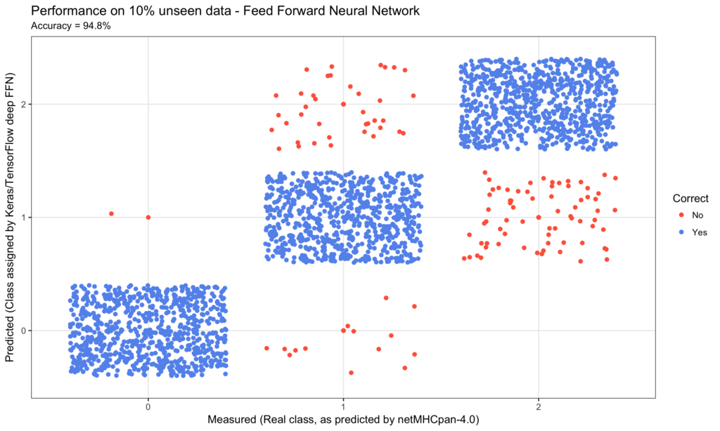
title = 'Efficiency on 10% unseen knowledge - Feed Ahead Neural Community'
xlab  = 'Measured (Actual class, as predicted by netMHCpan-4.0)'
ylab  = 'Predicted (Class assigned by Keras/TensorFlow deep FFN)'
outcomes %>%
  ggplot(aes(x = y_pred, y = y_real, color = Appropriate)) +
  geom_point() +
  ggtitle(label = title, subtitle = paste0("Accuracy = ", acc,"%")) +
  xlab(xlab) +
  ylab(ylab) +
  scale_color_manual(labels = c('No', 'Sure'),
                     values = c('tomato','cornflowerblue')) +
  geom_jitter() +
  theme_bw()

The ultimate consequence was a efficiency on the ten% unseen knowledge of simply wanting 95% accuracy.

Convolutional Neural Community

With a purpose to check a extra advanced structure, we additionally applied a Convolutional Neural Community. To make the comparability, we repeated the info preparation as described above and solely modified the structure by together with a single 2nd convolutional layer after which feeding that into the identical structure because the FFN above:

mannequin <- keras_model_sequential() %>%
  layer_conv_2d(filters = 32, kernel_size = c(3,3), activation = 'relu',
                input_shape = c(9, 20, 1)) %>%
  layer_dropout(fee = 0.25) %>% 
  layer_flatten() %>% 
  layer_dense(models  = 180, activation = 'relu') %>% 
  layer_dropout(fee = 0.4) %>% 
  layer_dense(models  = 90, activation  = 'relu') %>%
  layer_dropout(fee = 0.3) %>%
  layer_dense(models  = 3, activation   = 'softmax')

This resulted in a efficiency on the ten% unseen knowledge of 92% accuracy.

One might need anticipated the CNN to have the ability to higher seize the data within the peptide ‘photos’. There may be nonetheless a vital distinction between the peptide ‘photos’ and the e.g. MNIST dataset. The peptide ‘photos’ don’t comprise edges and spatially organized steady buildings, moderately they’re a set of pixels with p2 at all times at p2 and likewise for p9, that are determinants for binding.

Random Forest

Understanding that deep ;incomes just isn’t essentially the best software for all prediction duties, we additionally created a random forest mannequin on the very same knowledge utilizing the randomForest bundle.

The x and y coaching knowledge was ready barely totally different utilizing PepTools::pep_encode_mat

# Setup coaching knowledge
goal  <- 'prepare'
x_train <- pep_dat %>% filter(data_type==goal) %>% pull(peptide) %>%
  pep_encode_mat %>% choose(-peptide)
y_train <- pep_dat %>% filter(data_type==goal) %>% pull(label_num) %>% issue

# Setup check knowledge
goal <- 'check'
x_test <- pep_dat %>% filter(data_type==goal) %>% pull(peptide) %>%
  pep_encode_mat %>% choose(-peptide)
y_test <- pep_dat %>% filter(data_type==goal) %>% pull(label_num) %>% issue

The random forest mannequin was then run utilizing 100 bushes like so:

rf_classifier <- randomForest(x = x_train, y = y_train, ntree = 100)

The outcomes of the mannequin had been collected as follows:

y_pred    <- predict(rf_classifier, x_test)
n_correct <- table(noticed = y_test, predicted = y_pred) %>% diag %>% sum
acc       <- (n_correct / length(y_test)) %>% round(3) * 100
outcomes   <- tibble(y_real  = y_test,
                   y_pred  = y_pred,
                   Appropriate = ifelse(y_real == y_pred,"sure","no") %>% issue)

We are able to then visualize the efficiency as we did with the FFN and the CNN:

title = "Efficiency on 10% unseen knowledge - Random Forest"
xlab  = "Measured (Actual class, as predicted by netMHCpan-4.0)"
ylab  = "Predicted (Class assigned by random forest)"
f_out = "plots/03_rf_01_results_3_by_3_confusion_matrix.png"
outcomes %>%
  ggplot(aes(x = y_pred, y = y_real, color = Appropriate)) +
  geom_point() +
  xlab(xlab) +
  ylab(ylab) +
  ggtitle(label = title, subtitle = paste0("Accuracy = ", acc,"%")) +
  scale_color_manual(labels = c('No', 'Sure'),
                     values = c('tomato','cornflowerblue')) +
  geom_jitter() +
  theme_bw()

Conclusion

On this submit you’ve gotten been proven how we construct 3 fashions: A Feed Ahead Neural Community (FFN), a Convolutional Neural Community (CNN) and a Random Forest (RF). Utilizing the identical knowledge, we obtained performances of ~95%, ~92% and ~82% for the FFN, CNN and RF respectively. The R-code for these fashions can be found right here:

It’s evident that the deep studying fashions seize the data within the system significantly better than the random forest mannequin. Nonetheless, the CNN mannequin didn’t not carry out in addition to the easy FFN. This illustrates one of many pitfalls of deep studying – blind alleys. There are an enormous variety of architectures out there, and when mixed with hyperparameter tuning the potential mannequin house is breathtakingly massive.

To extend the probability of discovering structure and the best hyper-parameters you will need to know and perceive the info you might be modeling. Additionally, if potential embody a number of sources of knowledge. For the case of peptide-MHC interplay, we embody not solely info of the energy of the binding as measured within the laboratory, but in addition info from precise human cells, the place peptide-MHC complexes are extracted and analysed.

It needs to be famous that once we construct fashions within the analysis group, a number of work goes into creating balanced coaching and check units. Fashions are additionally educated and evaluated utilizing cross-validation, often 5-fold. We then save every of the 5 fashions and create an ensemble prediction – wisdom-of-the-crowd. We’re very cautious to avoiding overfitting as this after all decreases the fashions extrapolation efficiency.

There is no such thing as a doubt that deep studying already performs a serious position in unraveling the complexities of the human immune system and related ailments. With the discharge of TensorFlow by Google together with the keras and tensorflow R packages we now have the instruments out there in R to discover this frontier.

Primer on Most cancers Immunotherapy

Right here is an elaborated background on DNA, proteins and most cancers . Nonetheless, transient and simplified as that is naturally a massively advanced topic.

DNA

The cell is the fundamental unit of life. Every cell in our physique harbors ~2 meters (6 ft) of DNA, which is equivalent throughout all cells. DNA makes up the blue print for our physique – our genetic code – utilizing solely 4 nucleic acids (therefore the title DNA = DeoxyriboNucleic Acid). We are able to signify the genetic code, utilizing: a,c,g and t. Every cell carries ~3,200,000,000 of those letters, which represent the blue print for our complete physique. The letters are organised into ~20,000 genes and from the genes we get proteins. In Bioinformatics, we signify DNA sequences as repeats of the 4 nucleotides, e.g. ctccgacgaatttcatgttcagggatagct....

Proteins

Evaluating with a constructing – if DNA is the blue print of tips on how to assemble a constructing, then the proteins are the bricks, home windows, chimney, plumbing and so forth. Some proteins are structural (like a brick), whereas others are purposeful (like a window you’ll be able to open and shut). All ~100,000 proteins in our physique are made by of solely 20 small molecules referred to as amino acids. Like with DNA, we will signify these 20 amino acids utilizing: A,R,N,D,C,Q,E,G,H,I,L,Ok,M,F,P,S,T,W,Y and V (observe lowercase for DNA and uppercase for amino acids). The typical measurement of a protein within the human physique ~300 amino acids and the sequence is the mixture of the 20 amino acids making up the protein written consecutively, e.g.: MRYEMGYWTAFRRDCRCTKSVPSQWEAADN.... The attentive reader will discover, that I discussed ~20,000 genes, from which we get ~100,000 proteins. That is because of the DNA in a single gene having the ability to take part other ways and thus produce multiple protein.

Peptides

A peptide is a small fragment of a protein of size ~5-15 amino acids. MHCI predominantly binds peptides containing 9 amino acids – A so referred to as 9-mer. Peptides play a vital position within the monitoring of cells in our physique by the human immune system. The info used on this use case consist solely of 9-mers.

The Human Immune System

Inside every cell, proteins are consistently being produced from DNA. So as to not muddle the cell, proteins are additionally consistently damaged down into peptides that are then recycled to provide new proteins. A few of these peptides are caught by a system and certain to MHCI (Main Histocompatibility Advanced sort 1, MHCI) and transported from within the cell to the surface, the place the peptide is displayed. The viewer of this show is the human immune system. Particular immune cells (T-cells) patrol the physique, searching for cells displaying surprising peptides. If a displayed peptide is surprising, the T-cells will terminate the cell. The T-cells have been educated to acknowledge international peptides (non-self) and ignore peptides which originate from our personal physique (self). That is the hallmark of the immune system – Defending us by distinguishing self from non-self. I the immune system just isn’t lively sufficient and thus fails to acknowledge non-self arising from an an infection it’s doubtlessly deadly. However if the immune system is just too lively and begins recognizing not solely non-self, but in addition self, you get autoimmune illness, which likewise is doubtlessly deadly.

Most cancers

Most cancers arises when errors (mutations) happen contained in the cell, leading to modified proteins. Which means that if the unique protein was e.g. MRYEMGYWTAFRRDCRCTKSVPSQWEAADN..., then the brand new misguided protein might be e.g. MRYEMGYWTAFRRDCRCTKSVPSQWEAADR.... The results of that is that the peptide displayed on the cell floor is altered. The T-cells will now acknowledge the peptide as surprising and terminate the cell. Nonetheless, the setting round a most cancers tumor could be very hostile to the T-cells, that are supposed to acknowledge and terminate the cell.

Most cancers Immunotherapy goals at taking a pattern of the tumor and isolate the T-cells, develop them in nice numbers after which reintroduce them into the physique. Now, regardless of the hostile setting across the tumor, sheer numbers consequence within the T-cells out competing the tumor. A particular department of most cancers immunotherapy goals at introducing T-cells, which have been specifically engineered to acknowledge a tumor. Nonetheless, on this case it’s of utmost significance to make sure that the T-cell does certainly acknowledge the tumor and nothing else than the tumor. If launched T-cells acknowledge wholesome tissue, the result might be deadly. It’s due to this fact extraordinarily essential to grasp the molecular interplay between the sick cell, i.e. the peptide and the MHCI, and the T-cell.

Our peptide classification model illustrates how deep studying is being utilized to extend our understanding of the molecular interactions governing the activation of the T-cells.