Classifying bodily exercise from smartphone knowledge
Introduction
On this submit we’ll describe tips on how to use smartphone accelerometer and gyroscope knowledge to foretell the bodily actions of the people carrying the telephones. The information used on this submit comes from the Smartphone-Based Recognition of Human Activities and Postural Transitions Data Set distributed by the College of California, Irvine. Thirty people had been tasked with performing varied fundamental actions with an hooked up smartphone recording motion utilizing an accelerometer and gyroscope.
Earlier than we start, let’s load the varied libraries that we’ll use within the evaluation:
library(keras)     # Neural Networks
library(tidyverse) # Knowledge cleansing / Visualization
library(knitr)     # Desk printing
library(rmarkdown) # Misc. output utilities
library(ggridges)  # Visualization
Actions dataset
The information used on this submit come from the Smartphone-Based Recognition of Human Activities and Postural Transitions Data Set(Reyes-Ortiz et al. 2016) distributed by the College of California, Irvine.
When downloaded from the hyperlink above, the information incorporates two completely different ‘elements.’ One which has been pre-processed utilizing varied characteristic extraction strategies corresponding to fast-fourier remodel, and one other RawData part that merely provides the uncooked X,Y,Z instructions of an accelerometer and gyroscope. None of the usual noise filtering or characteristic extraction utilized in accelerometer knowledge has been utilized. That is the information set we’ll use.
The motivation for working with the uncooked knowledge on this submit is to assist the transition of the code/ideas to time sequence knowledge in much less well-characterized domains. Whereas a extra correct mannequin might be made by using the filtered/cleaned knowledge supplied, the filtering and transformation can fluctuate enormously from job to job; requiring plenty of handbook effort and area information. One of many stunning issues about deep studying is the characteristic extraction is discovered from the information, not exterior information.
Exercise labels
The information has integer encodings for the actions which, whereas not essential to the mannequin itself, are useful to be used to see. Let’s load them first.
activityLabels <- learn.desk("knowledge/activity_labels.txt",
                             col.names = c("quantity", "label"))

activityLabels %>% kable(align = c("c", "l"))| 1 | WALKING |
| 2 | WALKING_UPSTAIRS |
| 3 | WALKING_DOWNSTAIRS |
| 4 | SITTING |
| 5 | STANDING |
| 6 | LAYING |
| 7 | STAND_TO_SIT |
| 8 | SIT_TO_STAND |
| 9 | SIT_TO_LIE |
| 10 | LIE_TO_SIT |
| 11 | STAND_TO_LIE |
| 12 | LIE_TO_STAND |
Subsequent, we load within the labels key for the RawData. This file is an inventory of all the observations, or particular person exercise recordings, contained within the knowledge set. The important thing for the columns is taken from the information README.txt.
Column 1: experiment quantity ID,
Column 2: person quantity ID,
Column 3: exercise quantity ID
Column 4: Label begin level
Column 5: Label finish level
The beginning and finish factors are in variety of sign log samples (recorded at 50hz).
Let’s check out the primary 50 rows:
labels <- learn.desk(
  "knowledge/RawData/labels.txt",
  col.names = c("experiment", "userId", "exercise", "startPos", "endPos")
)

labels %>%
  head(50) %>%
  paged_table()
File names
Subsequent, let’s have a look at the precise information of the person knowledge supplied to us in RawData/
dataFiles <- record.information("knowledge/RawData")
dataFiles %>% head()
[1] "acc_exp01_user01.txt" "acc_exp02_user01.txt"
[3] "acc_exp03_user02.txt" "acc_exp04_user02.txt"
[5] "acc_exp05_user03.txt" "acc_exp06_user03.txt"
There’s a three-part file naming scheme. The primary half is the kind of knowledge the file incorporates: both acc for accelerometer or gyro for gyroscope. Subsequent is the experiment quantity, and final is the person Id for the recording. Let’s load these right into a dataframe for ease of use later.
fileInfo <- data_frame(
  filePath = dataFiles
) %>%
  filter(filePath != "labels.txt") %>%
  separate(filePath, sep = '_',
           into = c("sort", "experiment", "userId"),
           take away = FALSE) %>%
  mutate(
    experiment = str_remove(experiment, "exp"),
    userId = str_remove_all(userId, "person|.txt")
  ) %>%
  unfold(sort, filePath)

fileInfo %>% head() %>% kable()| 01 | 01 | acc_exp01_user01.txt | gyro_exp01_user01.txt |
| 02 | 01 | acc_exp02_user01.txt | gyro_exp02_user01.txt |
| 03 | 02 | acc_exp03_user02.txt | gyro_exp03_user02.txt |
| 04 | 02 | acc_exp04_user02.txt | gyro_exp04_user02.txt |
| 05 | 03 | acc_exp05_user03.txt | gyro_exp05_user03.txt |
| 06 | 03 | acc_exp06_user03.txt | gyro_exp06_user03.txt |
Studying and gathering knowledge
Earlier than we will do something with the information supplied we have to get it right into a model-friendly format. This implies we need to have an inventory of observations, their class (or exercise label), and the information similar to the recording.
To acquire this we’ll scan by way of every of the recording information current in dataFiles, search for what observations are contained within the recording, extract these recordings and return all the pieces to a simple to mannequin with dataframe.
# Learn contents of single file to a dataframe with accelerometer and gyro knowledge.
readInData <- operate(experiment, userId){
  genFilePath = operate(sort) {
    paste0("knowledge/RawData/", sort, "_exp",experiment, "_user", userId, ".txt")
  }

  bind_cols(
    learn.desk(genFilePath("acc"), col.names = c("a_x", "a_y", "a_z")),
    learn.desk(genFilePath("gyro"), col.names = c("g_x", "g_y", "g_z"))
  )
}

# Operate to learn a given file and get the observations contained alongside
# with their lessons.

loadFileData <- operate(curExperiment, curUserId) {

  # load sensor knowledge from file into dataframe
  allData <- readInData(curExperiment, curUserId)

  extractObservation <- operate(startPos, endPos){
    allData[startPos:endPos,]
  }

  # get commentary places on this file from labels dataframe
  dataLabels <- labels %>%
    filter(userId == as.integer(curUserId),
           experiment == as.integer(curExperiment))


  # extract observations as dataframes and save as a column in dataframe.
  dataLabels %>%
    mutate(
      knowledge = map2(startPos, endPos, extractObservation)
    ) %>%
    choose(-startPos, -endPos)
}

# scan by way of all experiment and userId combos and collect knowledge right into a dataframe.
allObservations <- map2_df(fileInfo$experiment, fileInfo$userId, loadFileData) %>%
  right_join(activityLabels, by = c("exercise" = "quantity")) %>%
  rename(activityName = label)

# cache work.
write_rds(allObservations, "allObservations.rds")
allObservations %>% dim()
Exploring the information
Now that we’ve all the information loaded together with the experiment, userId, and exercise labels, we will discover the information set.
Size of recordings
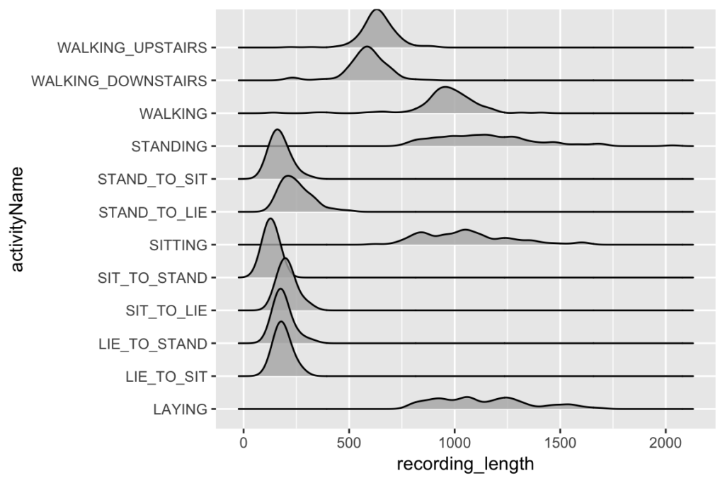
Let’s first have a look at the size of the recordings by exercise.
allObservations %>%
  mutate(recording_length = map_int(knowledge,nrow)) %>%
  ggplot(aes(x = recording_length, y = activityName)) +
  geom_density_ridges(alpha = 0.8)
The actual fact there’s such a distinction in size of recording between the completely different exercise varieties requires us to be a bit cautious with how we proceed. If we practice the mannequin on each class directly we’re going to must pad all of the observations to the size of the longest, which would go away a big majority of the observations with an enormous proportion of their knowledge being simply padding-zeros. Due to this, we’ll match our mannequin to only the most important ‘group’ of observations size actions, these embody STAND_TO_SIT, STAND_TO_LIE, SIT_TO_STAND, SIT_TO_LIE, LIE_TO_STAND, and LIE_TO_SIT.
An attention-grabbing future course could be making an attempt to make use of one other structure corresponding to an RNN that may deal with variable size inputs and coaching it on all the information. Nevertheless, you’d run the danger of the mannequin studying merely that if the commentary is lengthy it’s most definitely one of many 4 longest lessons which might not generalize to a state of affairs the place you had been working this mannequin on a real-time-stream of knowledge.
Filtering actions
Based mostly on our work from above, let’s subset the information to only be of the actions of curiosity.
desiredActivities <- c(
  "STAND_TO_SIT", "SIT_TO_STAND", "SIT_TO_LIE",
  "LIE_TO_SIT", "STAND_TO_LIE", "LIE_TO_STAND"
)

filteredObservations <- allObservations %>%
  filter(activityName %in% desiredActivities) %>%
  mutate(observationId = 1:n())

filteredObservations %>% paged_table()
So after our aggressive pruning of the information we can have a decent quantity of knowledge left upon which our mannequin can be taught.
Coaching/testing cut up
Earlier than we go any additional into exploring the information for our mannequin, in an try to be as honest as doable with our efficiency measures, we have to cut up the information right into a practice and take a look at set. Since every person carried out all actions simply as soon as (except one who solely did 10 of the 12 actions) by splitting on userId we’ll make sure that our mannequin sees new individuals completely once we take a look at it.
# get all customers
userIds <- allObservations$userId %>% distinctive()

# randomly select 24 (80% of 30 people) for coaching
set.seed(42) # seed for reproducibility
trainIds <- pattern(userIds, measurement = 24)

# set the remainder of the customers to the testing set
testIds <- setdiff(userIds,trainIds)

# filter knowledge.
trainData <- filteredObservations %>%
  filter(userId %in% trainIds)

testData <- filteredObservations %>%
  filter(userId %in% testIds)
Visualizing actions
Now that we’ve trimmed our knowledge by eradicating actions and splitting off a take a look at set, we will truly visualize the information for every class to see if there’s any instantly discernible form that our mannequin could possibly decide up on.
First let’s unpack our knowledge from its dataframe of one-row-per-observation to a tidy model of all of the observations.
unpackedObs <- 1:nrow(trainData) %>%
  map_df(operate(rowNum){
    dataRow <- trainData[rowNum, ]
    dataRow$knowledge[[1]] %>%
      mutate(
        activityName = dataRow$activityName,
        observationId = dataRow$observationId,
        time = 1:n() )
  }) %>%
  collect(studying, worth, -time, -activityName, -observationId) %>%
  separate(studying, into = c("sort", "course"), sep = "_") %>%
  mutate(sort = ifelse(sort == "a", "acceleration", "gyro"))
Now we’ve an unpacked set of our observations, let’s visualize them!
unpackedObs %>%
  ggplot(aes(x = time, y = worth, coloration = course)) +
  geom_line(alpha = 0.2) +
  geom_smooth(se = FALSE, alpha = 0.7, measurement = 0.5) +
  facet_grid(sort ~ activityName, scales = "free_y") +
  theme_minimal() +
  theme( axis.textual content.x = element_blank() )
So at the very least within the accelerometer knowledge patterns positively emerge. One would think about that the mannequin might have bother with the variations between LIE_TO_SIT and LIE_TO_STAND as they’ve the same profile on common. The identical goes for SIT_TO_STAND and STAND_TO_SIT.
Preprocessing
Earlier than we will practice the neural community, we have to take a few steps to preprocess the information.
Padding observations
First we’ll resolve what size to pad (and truncate) our sequences to by discovering what the 98th percentile size is. By not utilizing the very longest commentary size this can assist us keep away from extra-long outlier recordings messing up the padding.
padSize <- trainData$knowledge %>%
  map_int(nrow) %>%
  quantile(p = 0.98) %>%
  ceiling()
padSize
98%
334
Now we merely must convert our record of observations to matrices, then use the tremendous useful pad_sequences() operate in Keras to pad all observations and switch them right into a 3D tensor for us.
convertToTensor <- . %>%
  map(as.matrix) %>%
  pad_sequences(maxlen = padSize)

trainObs <- trainData$knowledge %>% convertToTensor()
testObs <- testData$knowledge %>% convertToTensor()

dim(trainObs)
[1] 286 334 6Fantastic, we now have our knowledge in a pleasant neural-network-friendly format of a 3D tensor with dimensions (<num obs>, <sequence size>, <channels>).
One-hot encoding
There’s one very last thing we have to do earlier than we will practice our mannequin, and that’s flip our commentary lessons from integers into one-hot, or dummy encoded, vectors. Fortunately, once more Keras has provided us with a really useful operate to do exactly this.
oneHotClasses <- . %>%
  {. - 7} %>%        # deliver integers right down to 0-6 from 7-12
  to_categorical() # One-hot encode

trainY <- trainData$exercise %>% oneHotClasses()
testY <- testData$exercise %>% oneHotClasses()
Modeling
Structure
Since we’ve temporally dense time-series knowledge we’ll make use of 1D convolutional layers. With temporally-dense knowledge, an RNN has to be taught very lengthy dependencies to be able to decide up on patterns, CNNs can merely stack a couple of convolutional layers to construct sample representations of considerable size. Since we’re additionally merely searching for a single classification of exercise for every commentary, we will simply use pooling to ‘summarize’ the CNNs view of the information right into a dense layer.
Along with stacking two layer_conv_1d() layers, we’ll use batch norm and dropout (the spatial variant(Tompson et al. 2014) on the convolutional layers and standard on the dense) to regularize the community.
input_shape <- dim(trainObs)[-1]
num_classes <- dim(trainY)[2]

filters <- 24     # variety of convolutional filters to be taught
kernel_size <- 8  # what number of time-steps every conv layer sees.
dense_size <- 48  # measurement of our penultimate dense layer.

# Initialize mannequin
mannequin <- keras_model_sequential()
mannequin %>%
  layer_conv_1d(
    filters = filters,
    kernel_size = kernel_size,
    input_shape = input_shape,
    padding = "legitimate",
    activation = "relu"
  ) %>%
  layer_batch_normalization() %>%
  layer_spatial_dropout_1d(0.15) %>%
  layer_conv_1d(
    filters = filters/2,
    kernel_size = kernel_size,
    activation = "relu",
  ) %>%
  # Apply common pooling:
  layer_global_average_pooling_1d() %>%
  layer_batch_normalization() %>%
  layer_dropout(0.2) %>%
  layer_dense(
    dense_size,
    activation = "relu"
  ) %>%
  layer_batch_normalization() %>%
  layer_dropout(0.25) %>%
  layer_dense(
    num_classes,
    activation = "softmax",
    title = "dense_output"
  )

abstract(mannequin)
______________________________________________________________________
Layer (sort)                   Output Form                Param #
======================================================================
conv1d_1 (Conv1D)              (None, 327, 24)             1176
______________________________________________________________________
batch_normalization_1 (BatchNo (None, 327, 24)             96
______________________________________________________________________
spatial_dropout1d_1 (SpatialDr (None, 327, 24)             0
______________________________________________________________________
conv1d_2 (Conv1D)              (None, 320, 12)             2316
______________________________________________________________________
global_average_pooling1d_1 (Gl (None, 12)                  0
______________________________________________________________________
batch_normalization_2 (BatchNo (None, 12)                  48
______________________________________________________________________
dropout_1 (Dropout)            (None, 12)                  0
______________________________________________________________________
dense_1 (Dense)                (None, 48)                  624
______________________________________________________________________
batch_normalization_3 (BatchNo (None, 48)                  192
______________________________________________________________________
dropout_2 (Dropout)            (None, 48)                  0
______________________________________________________________________
dense_output (Dense)           (None, 6)                   294
======================================================================
Complete params: 4,746
Trainable params: 4,578
Non-trainable params: 168
______________________________________________________________________
Coaching
Now we will practice the mannequin utilizing our take a look at and coaching knowledge. Be aware that we use callback_model_checkpoint() to make sure that we save solely the very best variation of the mannequin (fascinating since in some unspecified time in the future in coaching the mannequin might start to overfit or in any other case cease enhancing).
# Compile mannequin
mannequin %>% compile(
  loss = "categorical_crossentropy",
  optimizer = "rmsprop",
  metrics = "accuracy"
)

trainHistory <- mannequin %>%
  match(
    x = trainObs, y = trainY,
    epochs = 350,
    validation_data = record(testObs, testY),
    callbacks = record(
      callback_model_checkpoint("best_model.h5",
                                save_best_only = TRUE)
    )
  )
The mannequin is studying one thing! We get a decent 94.4% accuracy on the validation knowledge, not dangerous with six doable lessons to select from. Let’s look into the validation efficiency just a little deeper to see the place the mannequin is messing up.
Analysis
Now that we’ve a educated mannequin let’s examine the errors that it made on our testing knowledge. We will load the very best mannequin from coaching primarily based upon validation accuracy after which have a look at every commentary, what the mannequin predicted, how excessive a likelihood it assigned, and the true exercise label.
# dataframe to get labels onto one-hot encoded prediction columns
oneHotToLabel <- activityLabels %>%
  mutate(quantity = quantity - 7) %>%
  filter(quantity >= 0) %>%
  mutate(class = paste0("V",quantity + 1)) %>%
  choose(-number)

# Load our greatest mannequin checkpoint
bestModel <- load_model_hdf5("best_model.h5")

tidyPredictionProbs <- bestModel %>%
  predict(testObs) %>%
  as_data_frame() %>%
  mutate(obs = 1:n()) %>%
  collect(class, prob, -obs) %>%
  right_join(oneHotToLabel, by = "class")

predictionPerformance <- tidyPredictionProbs %>%
  group_by(obs) %>%
  summarise(
    highestProb = max(prob),
    predicted = label[prob == highestProb]
  ) %>%
  mutate(
    fact = testData$activityName,
    right = fact == predicted
  )

predictionPerformance %>% paged_table()
First, let’s have a look at how ‘assured’ the mannequin was by if the prediction was right or not.
predictionPerformance %>%
  mutate(consequence = ifelse(right, 'Appropriate', 'Incorrect')) %>%
  ggplot(aes(highestProb)) +
  geom_histogram(binwidth = 0.01) +
  geom_rug(alpha = 0.5) +
  facet_grid(consequence~.) +
  ggtitle("Possibilities related to prediction by correctness")
Reassuringly it appears the mannequin was, on common, much less assured about its classifications for the wrong outcomes than the right ones. (Though, the pattern measurement is just too small to say something definitively.)
Let’s see what actions the mannequin had the toughest time with utilizing a confusion matrix.
predictionPerformance %>%
  group_by(fact, predicted) %>%
  summarise(rely = n()) %>%
  mutate(good = fact == predicted) %>%
  ggplot(aes(x = fact,  y = predicted)) +
  geom_point(aes(measurement = rely, coloration = good)) +
  geom_text(aes(label = rely),
            hjust = 0, vjust = 0,
            nudge_x = 0.1, nudge_y = 0.1) +
  guides(coloration = FALSE, measurement = FALSE) +
  theme_minimal()
We see that, because the preliminary visualization prompt, the mannequin had a little bit of bother with distinguishing between LIE_TO_SIT and LIE_TO_STAND lessons, together with the SIT_TO_LIE and STAND_TO_LIE, which even have related visible profiles.
Future instructions
The obvious future course to take this evaluation could be to aim to make the mannequin extra basic by working with extra of the provided exercise varieties. One other attention-grabbing course could be to not separate the recordings into distinct ‘observations’ however as an alternative maintain them as one streaming set of knowledge, very similar to an actual world deployment of a mannequin would work, and see how nicely a mannequin may classify streaming knowledge and detect modifications in exercise.
Gal, Yarin, and Zoubin Ghahramani. 2016. “Dropout as a Bayesian Approximation: Representing Mannequin Uncertainty in Deep Studying.” In Worldwide Convention on Machine Studying, 1050–9.
Graves, Alex. 2012. “Supervised Sequence Labelling.” In Supervised Sequence Labelling with Recurrent Neural Networks, 5–13. Springer.
Kononenko, Igor. 1989. “Bayesian Neural Networks.” Organic Cybernetics 61 (5). Springer: 361–70.
LeCun, Yann, Yoshua Bengio, and Geoffrey Hinton. 2015. “Deep Studying.” Nature 521 (7553). Nature Publishing Group: 436.
Reyes-Ortiz, Jorge-L, Luca Oneto, Albert Samà, Xavier Parra, and Davide Anguita. 2016. “Transition-Conscious Human Exercise Recognition Utilizing Smartphones.” Neurocomputing 171. Elsevier: 754–67.
Tompson, Jonathan, Ross Goroshin, Arjun Jain, Yann LeCun, and Christoph Bregler. 2014. “Environment friendly Object Localization Utilizing Convolutional Networks.” CoRR abs/1411.4280. http://arxiv.org/abs/1411.4280.