Neural type switch with keen execution and Keras
How would your summer season vacation’s images look had Edvard Munch painted them? (Maybe it’s higher to not know).
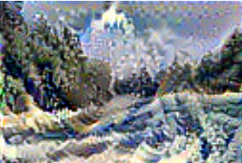
Let’s take a extra comforting instance: How would a pleasant, summarly river panorama look if painted by Katsushika Hokusai?
Fashion switch on pictures shouldn’t be new, however acquired a lift when Gatys, Ecker, and Bethge(Gatys, Ecker, and Bethge 2015) confirmed tips on how to efficiently do it with deep studying.
The principle concept is easy: Create a hybrid that could be a tradeoff between the content material picture we wish to manipulate, and a type picture we wish to imitate, by optimizing for maximal resemblance to each on the similar time.
When you’ve learn the chapter on neural type switch from Deep Learning with R, it’s possible you’ll acknowledge among the code snippets that observe.
Nevertheless, there is a vital distinction: This put up makes use of TensorFlow Eager Execution, permitting for an crucial means of coding that makes it simple to map ideas to code.
Similar to earlier posts on keen execution on this weblog, it is a port of a Google Colaboratory notebook that performs the identical job in Python.
As typical, please be sure you have the required bundle variations put in. And no want to repeat the snippets – you’ll discover the entire code among the many Keras examples.
Conditions
The code on this put up relies on the newest variations of a number of of the TensorFlow R packages. You possibly can set up these packages as follows:
install.packages(c("tensorflow", "keras", "tfdatasets"))You should also be sure that you are running the very latest version of TensorFlow (v1.10), which you can install like so:
library(tensorflow)
install_tensorflow()
There are additional requirements for using TensorFlow eager execution. First, we need to call tfe_enable_eager_execution() right at the beginning of the program. Second, we need to use the implementation of Keras included in TensorFlow, rather than the base Keras implementation.
Prerequisites behind us, let’s get started!
Input images
Here is our content image – replace by an image of your own:
# If you have enough memory on your GPU, no need to load the images
# at such small size.
# This is the size I found working for a 4G GPU.
img_shape <- c(128, 128, 3)

content_path <- "isar.jpg"

content_image <-  image_load(content_path, target_size = img_shape[1:2])
content_image %>%
  image_to_array() %>%
  `/`(., 255) %>%
  as.raster() %>%
  plot()
And right here’s the type mannequin, Hokusai’s The Nice Wave off Kanagawa, which you’ll obtain from Wikimedia Commons:

We create a wrapper that masses and preprocesses the enter pictures for us.
As we will probably be working with VGG19, a community that has been skilled on ImageNet, we have to remodel our enter pictures in the identical means that was used coaching it. Later, we’ll apply the inverse transformation to our mixture picture earlier than displaying it.
load_and_preprocess_image <- operate(path) {
  img <- image_load(path, target_size = img_shape[1:2]) %>%
    image_to_array() %>%
    k_expand_dims(axis = 1) %>%
    imagenet_preprocess_input()
}

deprocess_image <- operate(x) {
  x <- x[1, , ,]
  # Take away zero-center by imply pixel
  x[, , 1] <- x[, , 1] + 103.939
  x[, , 2] <- x[, , 2] + 116.779
  x[, , 3] <- x[, , 3] + 123.68
  # 'BGR'->'RGB'
  x <- x[, , c(3, 2, 1)]
  x[x > 255] <- 255
  x[x < 0] <- 0
  x[] <- as.integer(x) / 255
  x
}
Setting the scene
We’re going to use a neural community, however we gained’t be coaching it. Neural type switch is a bit unusual in that we don’t optimize the community’s weights, however again propagate the loss to the enter layer (the picture), so as to transfer it within the desired route.
We will probably be interested by two sorts of outputs from the community, similar to our two objectives.
Firstly, we wish to preserve the mixture picture much like the content material picture, on a excessive degree. In a convnet, higher layers map to extra holistic ideas, so we’re choosing a layer excessive up within the graph to match outputs from the supply and the mixture.
Secondly, the generated picture ought to “appear to be” the type picture. Fashion corresponds to decrease degree options like texture, shapes, strokes… So to match the mixture towards the type instance, we select a set of decrease degree conv blocks for comparability and mixture the outcomes.
content_layers <- c("block5_conv2")
style_layers <- c("block1_conv1",
                 "block2_conv1",
                 "block3_conv1",
                 "block4_conv1",
                 "block5_conv1")

num_content_layers <- length(content_layers)
num_style_layers <- length(style_layers)

get_model <- operate() {
  vgg <- application_vgg19(include_top = FALSE, weights = "imagenet")
  vgg$trainable <- FALSE
  style_outputs <- map(style_layers, operate(layer) vgg$get_layer(layer)$output)
  content_outputs <- map(content_layers, operate(layer) vgg$get_layer(layer)$output)
  model_outputs <- c(style_outputs, content_outputs)
  keras_model(vgg$enter, model_outputs)
}
Losses
When optimizing the enter picture, we are going to take into account three kinds of losses. Firstly, the content material loss: How completely different is the mixture picture from the supply? Right here, we’re utilizing the sum of the squared errors for comparability.
content_loss <- operate(content_image, goal) {
  k_sum(k_square(goal - content_image))
}
Our second concern is having the types match as intently as potential. Fashion is usually operationalized because the Gram matrix of flattened characteristic maps in a layer. We thus assume that type is said to how maps in a layer correlate with different.
We subsequently compute the Gram matrices of the layers we’re interested by (outlined above), for the supply picture in addition to the optimization candidate, and evaluate them, once more utilizing the sum of squared errors.
gram_matrix <- operate(x) {
  options <- k_batch_flatten(k_permute_dimensions(x, c(3, 1, 2)))
  gram <- k_dot(options, k_transpose(options))
  gram
}

style_loss <- operate(gram_target, mixture) {
  gram_comb <- gram_matrix(mixture)
  k_sum(k_square(gram_target - gram_comb)) /
    (4 * (img_shape[3] ^ 2) * (img_shape[1] * img_shape[2]) ^ 2)
}
Thirdly, we don’t need the mixture picture to look overly pixelated, thus we’re including in a regularization element, the whole variation within the picture:
total_variation_loss <- operate(picture) {
  y_ij  <- picture[1:(img_shape[1] - 1L), 1:(img_shape[2] - 1L),]
  y_i1j <- picture[2:(img_shape[1]), 1:(img_shape[2] - 1L),]
  y_ij1 <- picture[1:(img_shape[1] - 1L), 2:(img_shape[2]),]
  a <- k_square(y_ij - y_i1j)
  b <- k_square(y_ij - y_ij1)
  k_sum(k_pow(a + b, 1.25))
}
The tough factor is tips on how to mix these losses. We’ve reached acceptable outcomes with the next weightings, however be at liberty to mess around as you see match:
content_weight <- 100
style_weight <- 0.8
total_variation_weight <- 0.01
Get mannequin outputs for the content material and magnificence pictures
We’d like the mannequin’s output for the content material and magnificence pictures, however right here it suffices to do that simply as soon as.
We concatenate each pictures alongside the batch dimension, go that enter to the mannequin, and get again a listing of outputs, the place each component of the listing is a 4-d tensor. For the type picture, we’re within the type outputs at batch place 1, whereas for the content material picture, we want the content material output at batch place 2.
Within the beneath feedback, please word that the sizes of dimensions 2 and three will differ in the event you’re loading pictures at a distinct dimension.
get_feature_representations <-
  operate(mannequin, content_path, style_path) {

    # dim == (1, 128, 128, 3)
    style_image <-
      load_and_process_image(style_path) %>% k_cast("float32")
    # dim == (1, 128, 128, 3)
    content_image <-
      load_and_process_image(content_path) %>% k_cast("float32")
    # dim == (2, 128, 128, 3)
    stack_images <- k_concatenate(list(style_image, content_image), axis = 1)

    # size(model_outputs) == 6
    # dim(model_outputs[[1]]) = (2, 128, 128, 64)
    # dim(model_outputs[[6]]) = (2, 8, 8, 512)
    model_outputs <- mannequin(stack_images)

    style_features <-
      model_outputs[1:num_style_layers] %>%
      map(operate(batch) batch[1, , , ])
    content_features <-
      model_outputs[(num_style_layers + 1):(num_style_layers + num_content_layers)] %>%
      map(operate(batch) batch[2, , , ])

    list(style_features, content_features)
  }
Computing the losses
On each iteration, we have to go the mixture picture by means of the mannequin, get hold of the type and content material outputs, and compute the losses. Once more, the code is extensively commented with tensor sizes for straightforward verification, however please understand that the precise numbers presuppose you’re working with 128×128 pictures.
compute_loss <-
  operate(mannequin, loss_weights, init_image, gram_style_features, content_features) {

    c(style_weight, content_weight) %<-% loss_weights
    model_outputs <- mannequin(init_image)
    style_output_features <- model_outputs[1:num_style_layers]
    content_output_features <-
      model_outputs[(num_style_layers + 1):(num_style_layers + num_content_layers)]

    # type loss
    weight_per_style_layer <- 1 / num_style_layers
    style_score <- 0
    # dim(style_zip[[5]][[1]]) == (512, 512)
    style_zip <- transpose(list(gram_style_features, style_output_features))
    for (l in 1:length(style_zip)) {
      # for l == 1:
      # dim(target_style) == (64, 64)
      # dim(comb_style) == (1, 128, 128, 64)
      c(target_style, comb_style) %<-% style_zip[[l]]
      style_score <- style_score + weight_per_style_layer *
        style_loss(target_style, comb_style[1, , , ])
    }

    # content material loss
    weight_per_content_layer <- 1 / num_content_layers
    content_score <- 0
    content_zip <- transpose(list(content_features, content_output_features))
    for (l in 1:length(content_zip)) {
      # dim(comb_content) ==  (1, 8, 8, 512)
      # dim(target_content) == (8, 8, 512)
      c(target_content, comb_content) %<-% content_zip[[l]]
      content_score <- content_score + weight_per_content_layer *
        content_loss(comb_content[1, , , ], target_content)
    }

    # complete variation loss
    variation_loss <- total_variation_loss(init_image[1, , ,])

    style_score <- style_score * style_weight
    content_score <- content_score * content_weight
    variation_score <- variation_loss * total_variation_weight

    loss <- style_score + content_score + variation_score
    list(loss, style_score, content_score, variation_score)
  }
Computing the gradients
As quickly as we’ve the losses, acquiring the gradients of the general loss with respect to the enter picture is only a matter of calling tape$gradient on the GradientTape. Notice that the nested name to compute_loss, and thus the decision of the mannequin on our mixture picture, occurs contained in the GradientTape context.
compute_grads <-
  operate(mannequin, loss_weights, init_image, gram_style_features, content_features) {
    with(tf$GradientTape() %as% tape, {
      scores <-
        compute_loss(mannequin,
                     loss_weights,
                     init_image,
                     gram_style_features,
                     content_features)
    })
    total_loss <- scores[[1]]
    list(tape$gradient(total_loss, init_image), scores)
  }
Coaching section
Now it’s time to coach! Whereas the pure continuation of this sentence would have been “… the mannequin,” the mannequin we’re coaching right here shouldn’t be VGG19 (that one we’re simply utilizing as a instrument), however a minimal setup of simply:
- a
Variablethat holds our to-be-optimized picture - the loss capabilities we outlined above
- an optimizer that may apply the calculated gradients to the picture variable (
tf$practice$AdamOptimizer)
Under, we get the type options (of the type picture) and the content material characteristic (of the content material picture) simply as soon as, then iterate over the optimization course of, saving the output each 100 iterations.
In distinction to the unique article and the Deep Studying with R ebook, however following the Google pocket book as a substitute, we’re not utilizing L-BFGS for optimization, however Adam, as our aim right here is to supply a concise introduction to keen execution.
Nevertheless, you could possibly plug in one other optimization technique in the event you needed, changing
optimizer$apply_gradients(listing(tuple(grads, init_image)))
by an algorithm of your alternative (and naturally, assigning the results of the optimization to the Variable holding the picture).
run_style_transfer <- operate(content_path, style_path) {
  mannequin <- get_model()
  walk(mannequin$layers, operate(layer) layer$trainable = FALSE)

  c(style_features, content_features) %<-%
    get_feature_representations(mannequin, content_path, style_path)
  # dim(gram_style_features[[1]]) == (64, 64)
  gram_style_features <- map(style_features, operate(characteristic) gram_matrix(characteristic))

  init_image <- load_and_process_image(content_path)
  init_image <- tf$contrib$keen$Variable(init_image, dtype = "float32")

  optimizer <- tf$practice$AdamOptimizer(learning_rate = 1,
                                      beta1 = 0.99,
                                      epsilon = 1e-1)

  c(best_loss, best_image) %<-% list(Inf, NULL)
  loss_weights <- list(style_weight, content_weight)

  start_time <- Sys.time()
  global_start <- Sys.time()

  norm_means <- c(103.939, 116.779, 123.68)
  min_vals <- -norm_means
  max_vals <- 255 - norm_means

  for (i in seq_len(num_iterations)) {
    # dim(grads) == (1, 128, 128, 3)
    c(grads, all_losses) %<-% compute_grads(mannequin,
                                            loss_weights,
                                            init_image,
                                            gram_style_features,
                                            content_features)
    c(loss, style_score, content_score, variation_score) %<-% all_losses
    optimizer$apply_gradients(list(tuple(grads, init_image)))
    clipped <- tf$clip_by_value(init_image, min_vals, max_vals)
    init_image$assign(clipped)

    end_time <- Sys.time()

    if (k_cast_to_floatx(loss) < best_loss) {
      best_loss <- k_cast_to_floatx(loss)
      best_image <- init_image
    }

    if (i %% 50 == 0) {
      glue("Iteration: {i}") %>% print()
      glue(
        "Complete loss: {k_cast_to_floatx(loss)},
        type loss: {k_cast_to_floatx(style_score)},
        content material loss: {k_cast_to_floatx(content_score)},
        complete variation loss: {k_cast_to_floatx(variation_score)},
        time for 1 iteration: {(Sys.time() - start_time) %>% spherical(2)}"
      ) %>% print()

      if (i %% 100 == 0) {
        png(paste0("style_epoch_", i, ".png"))
        plot_image <- best_image$numpy()
        plot_image <- deprocess_image(plot_image)
        plot(as.raster(plot_image), major = glue("Iteration {i}"))
        dev.off()
      }
    }
  }

  glue("Complete time: {Sys.time() - global_start} seconds") %>% print()
  list(best_image, best_loss)
}
Able to run
Now, we’re prepared to begin the method:
c(best_image, best_loss) %<-% run_style_transfer(content_path, style_path)In our case, outcomes didn’t change a lot after ~ iteration 1000, and that is how our river panorama was wanting:

… undoubtedly extra inviting than had it been painted by Edvard Munch!
Conclusion
With neural type switch, some fiddling round could also be wanted till you get the end result you need. However as our instance exhibits, this doesn’t imply the code needs to be sophisticated. Moreover to being simple to know, keen execution additionally allows you to add debugging output, and step by means of the code line-by-line to test on tensor shapes.
Till subsequent time in our keen execution sequence!


