Unraveling the Regulation of Massive Numbers | by Sachin Date | Jul, 2023

The LLN is attention-grabbing as a lot for what it doesn’t say as for what it does

O n August 24, 1966, a gifted playwright by the title Tom Stoppard staged a play in Edinburgh, Scotland. The play had a curious title, “Rosencrantz and Guildenstern Are Dead.” Its central characters, Rosencrantz and Guildenstern, are childhood pals of Hamlet (of Shakespearean fame). The play opens with Guildenstern repeatedly tossing cash which preserve arising Heads. Every consequence makes Guildenstern’s money-bag lighter and Rosencrantz’s, heavier. Because the drumbeat of Heads continues with a pitiless persistence, Guildenstern is fearful. He worries if he’s secretly prepared every coin to come back up Heads as a self-inflicted punishment for some long-forgotten sin. Or if time stopped after the primary flip, and he and Rosencrantz are experiencing the identical consequence over and over.

Stoppard does an excellent job of exhibiting how the legal guidelines of chance are woven into our view of the world, into our sense of expectation, into the very material of human thought. When the 92nd flip additionally comes up as Heads, Guildenstern asks if he and Rosencrantz are throughout the management of an unnatural actuality the place the legal guidelines of chance now not function.

Guildenstern’s fears are after all unfounded. Granted, the probability of getting 92 Heads in a row is unimaginably small. Actually, it’s a decimal level adopted by 28 zeroes adopted by 2. Guildenstern is extra more likely to be hit on the top by a meteorite.

Guildenstern solely has to come back again the following day to flip one other sequence of 92 coin tosses and the consequence will nearly definitely be vastly totally different. If he have been to comply with this routine day-after-day, he’ll uncover that on most days the variety of Heads will roughly match the variety of tails. Guildenstern is experiencing an enchanting conduct of our universe generally known as the Regulation of Massive Numbers.

The LLN, as it’s known as, is available in two flavors: the weak and the sturdy. The weak LLN could be extra intuitive and simpler to narrate to. However it is usually straightforward to misread. I’ll cowl the weak model on this article and go away the dialogue on the sturdy model for a later article.

The weak Regulation of Massive Numbers considerations itself with the connection between the pattern imply and the inhabitants imply. I’ll clarify what it says in plain textual content:

Suppose you draw a random pattern of a sure measurement, say 100, from the inhabitants. By the way in which, make a psychological be aware of the time period pattern measurement. The measurement of the pattern is the ringmaster, the grand pooh-bah of this legislation. Now calculate the imply of this pattern and set it apart. Subsequent, repeat this course of many many occasions. What you’ll get is a set of imperfect means. The means are imperfect as a result of there’ll at all times be a ‘hole’, a delta, a deviation between them and the true inhabitants imply. Let’s assume you’ll tolerate a sure deviation. If you choose a pattern imply at random from this set of means, there will likely be an opportunity that absolutely the distinction between the pattern imply and the inhabitants imply will exceed your tolerance.

The weak Regulation of Massive Numbers says that the chance of this deviation’s exceeding your chosen stage of tolerance will shrink to zero because the pattern measurement grows to both infinity or to the scale of the inhabitants.

Regardless of how tiny is your chosen stage of tolerance, as you draw units of samples of ever growing measurement, it’ll change into more and more unlikely that the imply of a randomly chosen pattern from the set will exceed this tolerance.

To see how the weak LLN works we’ll run it by way of an instance. And for that, enable me, if you’ll, to take you to the chilly, brooding expanse of the Northeastern North Atlantic Ocean.

Each day, the Authorities of Eire publishes a dataset of water temperature measurements taken from the floor of the North East North Atlantic. This dataset incorporates tons of of hundreds of measurements of floor water temperature listed by latitude and longitude. As an illustration, the info for June 21, 2023 is as follows:

It’s sort of arduous to think about what eight hundred thousand floor temperature values appear to be. So let’s create a scatter plot to visualise this information. I’ve proven this plot under. The vacant white areas within the plot characterize Eire and the UK.

As a pupil of statistics, you’ll by no means have entry to the ‘inhabitants’. So that you’ll be appropriate in severely chiding me if I declare this inhabitants of 800,000 temperature measurements because the ‘inhabitants’. However bear with me for a short time. You’ll quickly see why, in our quest to grasp the LLN, it helps us to contemplate this information because the ‘inhabitants’.

So let’s assume that this information is — ahem…cough — the inhabitants. The typical floor water temperature throughout the 810219 places on this inhabitants of values is 17.25840 levels Celsius. 17.25840 is solely the typical of the 810K temperature measurements. We’ll designate this worth because the inhabitants imply, μ. Keep in mind this worth. You’ll must check with it typically.

Now suppose this inhabitants of 810219 values isn’t accessible to you. As an alternative, all you might have entry to is a meager little pattern of 20 random places drawn from this inhabitants. Right here’s one such random pattern:

The imply temperature of the pattern is 16.9452414 levels C. That is our pattern imply X_bar which is computed as follows:

X_bar = (X1 + X2 + X3 + … + X20) / 20

You possibly can simply as simply draw a second, a 3rd, certainly any variety of such random samples of measurement 20 from the identical inhabitants. Listed below are a couple of random samples for illustration:

A fast apart on what a random pattern actually is

Earlier than shifting forward, let’s pause a bit to get a sure diploma of perspective on the idea of a random pattern. It can make it simpler to grasp how the weak LLN works. And to amass this angle, I need to introduce you to the on line casino slot machine:

The slot machine proven above incorporates three slots. Each time you crank down the arm of the machine, the machine fills every slot with an image that the machine has chosen randomly from an internally maintained inhabitants of images similar to a listing of fruit photos. Now think about a slot machine with 20 slots named X1 by way of X20. Assume that the machine is designed to pick out values from a inhabitants of 810219 temperature measurements. While you pull down the arm, every one of many 20 slots — X1 by way of X20 — fills with a randomly chosen worth from the inhabitants of 810219 values. Due to this fact, X1 by way of X20 are random variables that may every maintain any worth from the inhabitants. Taken collectively they kind a random pattern. Put one other manner, every factor of a random pattern is itself a random variable.

X1 by way of X20 have a couple of attention-grabbing properties:

• The worth that X1 acquires is unbiased of the values that X2 through X20 purchase. The identical applies to X2, X3, …,X20. Thus X1 through X20 are unbiased random variables.
• As a result of X1, X2,…, X20 can every maintain any worth from the inhabitants, the imply of every of them is the inhabitants imply, μ. Utilizing the notation E() for expectation, we write this consequence as follows:
  E(X1) = E(X2) = … = E(X20) = μ.
• X1 through X20 have equivalent chance distributions.

Thus, X1, X2,…,X20 are unbiased, identically distributed (i.i.d.) random variables.

…and now we get again to exhibiting how the weak LLN works

Let’s compute the imply (denoted by X_bar) of this 20 factor pattern and set it apart. Now let’s as soon as once more crank down the machine’s arm and out will pop one other 20-element random pattern. We’ll compute its imply and set it apart too. If we repeat this course of one thousand occasions, we may have computed one thousand pattern means.

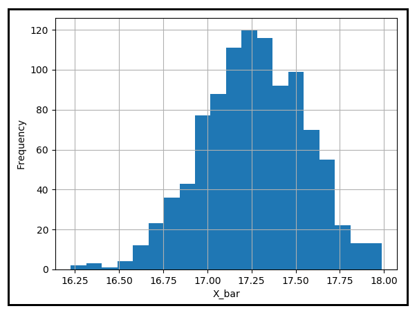
Right here’s a desk of 1000 pattern means computed this manner. We’ll designate them as X_bar_1 to X_bar_1000:

Now take into account the next assertion fastidiously:

For the reason that pattern imply is calculated from a random pattern, the pattern imply is itself a random variable.

At this level, in case you are sagely nodding your head and stroking your chin, it is vitally a lot the suitable factor to do. The conclusion that the pattern imply is a random variable is likely one of the most penetrating realizations one can have in statistics.

Discover additionally how every pattern imply within the desk above is a long way away from the inhabitants imply, μ. Let’s plot a histogram of those pattern means to see how they’re distributed round μ:

Many of the pattern means appear to lie near the inhabitants imply of 17.25840 levels Celsius. Nevertheless, there are some which might be significantly distant from μ. Suppose your tolerance for this distance is 0.25 levels Celsius. For those who have been to plunge your hand into this bucket of 1000 pattern means, seize whichever imply falls inside your grasp and pull it out. What would be the chance that absolutely the distinction between this imply and μ is the same as or larger than 0.25 levels C? To estimate this chance, you could rely the variety of pattern means which might be a minimum of 0.25 levels away from μ and divide this quantity by 1000.

Within the above desk, this rely occurs to be 422 and so the chance P(|X_bar — μ | ≥ 0.25) works out to be 422/1000 = 0.422

Let’s park this chance for a minute.

Now repeat all the above steps, however this time use a pattern measurement of 100 as a substitute of 20. So right here’s what you’ll do: draw 1000 random samples every of measurement 100, take the imply of every pattern, retailer away all these means, rely those which might be a minimum of 0.25 levels C away from μ, and divide this rely by 1000. If that sounded just like the labors of Hercules, you weren’t mistaken. So take a second to catch your breath. And as soon as you might be all caught up, discover under what you’ve got because the fruit on your labors.

The desk under incorporates the means from the 1000 random samples, every of measurement 100:

Out of those one thousand means, fifty-six means occur to deviate by least 0.25 levels C from μ. That offers you the chance that you just’ll run into such a imply as 56/1000 = 0.056. This chance is decidedly smaller than the 0.422 we computed earlier when the pattern measurement was solely 20.

For those who repeat this sequence of steps a number of occasions, every time with a distinct pattern measurement that will increase incrementally, you’re going to get your self a desk filled with possibilities. I’ve carried out this train for you by dialing up the pattern measurement from 10 by way of 490 in steps of 10. Right here’s the result:

Every row on this desk corresponds to 1000 totally different samples that I drew at random from the inhabitants of 810219 temperature measurements. The sample_size column mentions the scale of every of those 1000 samples. As soon as drawn, I took the imply of every pattern and counted those that have been a minimum of 0.25 levels C aside from μ. The num_exceeds_tolerance column mentions this rely. The chance column is num_exceeds_tolerance / sample_size.

Discover how this rely attenuates quickly because the pattern measurement will increase. And so does the corresponding chance P(|X_bar — μ | ≥ 0.25). By the point the pattern measurement reaches 320, the chance has decayed to zero. It blips as much as 0.001 often however that’s as a result of I’ve drawn a finite variety of samples. If every time I draw 10000 samples as a substitute of 1000, not solely will the occasional blips flatten out however the attenuation of possibilities can even change into smoother.

The next graph plots P(|X_bar — μ | ≥ 0.25) towards pattern measurement. It places in sharp reduction how the chance plunges to zero because the pattern measurement grows.

Instead of 0.25 levels C, what if you happen to selected a distinct tolerance — both a decrease or a better worth? Will the chance decay no matter your chosen stage of tolerance? The next household of plots illustrates the reply to this query.

Regardless of how frugal, how tiny, is your selection of the tolerance (ε), the chance P(|X_bar — μ | ≥ ε) will at all times converge to zero because the pattern measurement grows. That is the weak Regulation of Massive Numbers in motion.

The conduct of the weak LLN could be formally acknowledged as follows:

Suppose X1, X2, …, Xn are i.i.d. random variables that collectively kind a random pattern of measurement n. Suppose X_bar_n is the imply of this pattern. Suppose additionally that E(X1) = E(X2) = … = E(Xn) = μ. Then for any non-negative actual quantity ε the chance of X_bar_n being a minimum of ε away from μ tends to zero as the scale of the pattern tends to infinity. The next beautiful equation captures this conduct:

Over the 310 yr historical past of this legislation, mathematicians have been in a position to progressively chill out the requirement that X1 by way of Xn be unbiased and identically distributed whereas nonetheless preserving the spirit of the legislation.

The precept of “convergence in chance”, the “plim” notation, and the artwork of claiming actually necessary issues in actually few phrases

The actual fashion of converging to some worth utilizing chance because the technique of transport is known as convergence in chance. On the whole, it’s acknowledged as follows:

Within the above equation, X_n and X are random variables. ε is a non-negative actual quantity. The equation says that as n tends to infinity, X_n converges in chance to X.

All through the immense expanse of statistics, you’ll preserve working right into a quietly unassuming notation known as plim. It’s pronounced ‘p lim’, or ‘plim’ (just like the phrase ‘ plum’ however with in ‘i’), or chance restrict. plim is the brief kind manner of claiming {that a} measure such because the imply converges in chance to a selected worth. Utilizing plim, the weak Regulation of Massive Numbers could be acknowledged pithily as follows:

Or just as:

The brevity of notation isn’t the least shocking. Mathematicians are drawn to brevity like bees to nectar. In the case of conveying profound truths, arithmetic may nicely be essentially the most ink-efficient discipline. And inside this efficiency-obsessed discipline, plim occupies podium place. You’ll wrestle to unearth as profound an idea as plim expressed in lesser quantity of ink, or electrons.

However wrestle no extra. If the laconic great thing about plim left you wanting for extra, right here’s one other, probably much more environment friendly, notation that conveys the identical that means as plim:

On the prime of this text, I discussed that the weak Regulation of Massive Numbers is noteworthy for what it doesn’t say as a lot as for what it does say. Let me clarify what I imply by that. The weak LLN is usually misinterpreted to imply that because the pattern measurement will increase, its imply approaches the inhabitants imply or varied generalizations of that concept. As we noticed, such concepts in regards to the weak LLN harbor no attachment to actuality.

Actually, let’s bust a few myths relating to the weak LLN instantly.

MYTH #1: Because the pattern measurement grows, the pattern imply tends to the inhabitants imply.

That is fairly probably essentially the most frequent misinterpretation of the weak LLN. Nevertheless, the weak LLN makes no such assertion. To see why that’s, take into account the next state of affairs: you might have managed to get your arms round a extremely massive pattern. Whilst you gleefully admire your achievement, you also needs to pose your self the next questions: Simply because your pattern is massive, should it even be well-balanced? What’s stopping nature from sucker punching you with an enormous pattern that incorporates an equally big quantity of bias? The reply is completely nothing! Actually, isn’t that what occurred to Guildenstern along with his sequence of 92 Heads? It was, in any case, a very random pattern! If it simply so occurs to have a big bias, then regardless of the massive pattern measurement, the bias will blast away the pattern imply to some extent that’s distant from the true inhabitants worth. Conversely, a small pattern can show to be exquisitely well-balanced. The purpose is, because the pattern measurement will increase, the pattern imply isn’t assured to dutifully advance towards the inhabitants imply. Nature doesn’t present such pointless ensures.

MYTH #2: Because the pattern measurement will increase, just about the whole lot in regards to the pattern — its median, its variance, its customary deviation — converges to the inhabitants values of the identical.

This sentence is 2 myths bundled into one easy-to-carry package deal. Firstly, the weak LLN postulates a convergence in chance, not in worth. Secondly, the weak LLN applies to the convergence in chance of solely the pattern imply, not another statistic. The weak LLN doesn’t deal with the convergence of different measures such because the median, variance, or customary deviation.

It’s one factor to state the weak LLN, and even display the way it works utilizing real-world information. However how are you going to ensure that it at all times works? Are there circumstances wherein it is going to play spoilsport — conditions wherein the pattern imply merely doesn’t converge in chance to the inhabitants worth? To know that, you could show the weak LLN and, in doing so, exactly outline the circumstances wherein it is going to apply.

It so occurs that the weak LLN has a deliciously mouth-watering proof that makes use of as considered one of its components, the endlessly tantalizing Chebyshev’s Inequality. If that whets your urge for food, keep tuned for my subsequent article on the proof of the weak Regulation of Massive Numbers.

It is going to be rude to take go away off this subject with out assuaging our buddy Guildenstern’s worries. Let’s develop an appreciation for simply how unquestionably unlikely a consequence it was that he skilled. We’ll simulate the act of tossing 92 unbiased cash utilizing a pseudo-random generator. Heads will likely be encoded as 1 and tails as 0. We’ll document the imply worth of the 92 outcomes. The imply worth is the fraction of occasions that the coin got here up Heads. We’ll repeat this experiment ten thousand occasions to acquire ten thousand technique of 92 coin tosses, and we’ll plot their frequency distribution. After finishing this train, we are going to get the next sort of histogram plot:

We see that a lot of the pattern means are grouped across the inhabitants imply of 0.5. Guildenstern’s consequence — getting 92 Heads in a row —is an exceptionally unlikely consequence. Due to this fact, the frequency of this consequence can be vanishingly small. However opposite to Guildenstern’s fears, there’s nothing unnatural in regards to the consequence and the legal guidelines of chance proceed to function with their regular gusto. Guildenstern’s consequence is solely lurking contained in the distant areas of the left tail of the plot, ready with infinite endurance to pounce upon some luckless coin-flipper whose solely mistake was to be unimaginably unfortunate.