Posit AI Weblog: TensorFlow characteristic columns: Remodeling your knowledge recipes-style
It’s 2019; nobody doubts the effectiveness of deep studying in laptop imaginative and prescient. Or pure language processing. With “regular,” Excel-style, a.okay.a. tabular knowledge nevertheless, the state of affairs is completely different.
Mainly there are two circumstances: One, you could have numeric knowledge solely. Then, creating the community is simple, and all can be about optimization and hyperparameter search. Two, you could have a mixture of numeric and categorical knowledge, the place categorical could possibly be something from ordered-numeric to symbolic (e.g., textual content). On this latter case, with categorical knowledge getting into the image, there may be an especially good concept you can also make use of: embed what are equidistant symbols right into a high-dimensional, numeric illustration. In that new illustration, we are able to outline a distance metric that permits us to make statements like “biking is nearer to operating than to baseball,” or “😃 is nearer to 😂 than to 😠.” When not coping with language knowledge, this system is known as entity embeddings.
Good as this sounds, why don’t we see entity embeddings used on a regular basis? Properly, making a Keras community that processes a mixture of numeric and categorical knowledge used to require a little bit of an effort. With TensorFlow’s new characteristic columns, usable from R via a mix of tfdatasets and keras, there’s a a lot simpler option to obtain this. What’s extra, tfdatasets follows the favored recipes idiom to initialize, refine, and apply a characteristic specification %>%-style. And eventually, there are ready-made steps for bucketizing a numeric column, or hashing it, or creating crossed columns to seize interactions.
This publish introduces characteristic specs ranging from a situation the place they don’t exist: mainly, the established order till very lately. Think about you could have a dataset like that from the Porto Seguro car insurance competition the place a number of the columns are numeric, and a few are categorical. You wish to practice a completely related community on it, with all categorical columns fed into embedding layers. How will you try this? We then distinction this with the characteristic spec method, which makes issues rather a lot simpler – particularly when there’s lots of categorical columns.
In a second utilized instance, we reveal the usage of crossed columns on the rugged dataset from Richard McElreath’s rethinking bundle. Right here, we additionally direct consideration to some technical particulars which are value figuring out about.
Mixing numeric knowledge and embeddings, the pre-feature-spec method
Our first instance dataset is taken from Kaggle. Two years in the past, Brazilian automotive insurance coverage firm Porto Seguro requested contributors to foretell how likely it is a car owner will file a claim based mostly on a mixture of traits collected in the course of the earlier yr. The dataset is relatively massive – there are ~ 600,000 rows within the coaching set, with 57 predictors. Amongst others, options are named in order to point the kind of the info – binary, categorical, or steady/ordinal.
Whereas it’s frequent in competitions to attempt to reverse-engineer column meanings, right here we simply make use of the kind of the info, and see how far that will get us.
Concretely, this implies we wish to
- use binary options simply the best way they’re, as zeroes and ones,
- scale the remaining numeric options to imply 0 and variance 1, and
- embed the explicit variables (each by itself).
We’ll then outline a dense community to foretell goal, the binary final result. So first, let’s see how we may get our knowledge into form, in addition to construct up the community, in a “handbook,” pre-feature-columns method.
When loading libraries, we already use the variations we’ll want very quickly: Tensorflow 2 (>= beta 1), and the event (= Github) variations of tfdatasets and keras:
On this first model of making ready the info, we make our lives simpler by assigning completely different R sorts, based mostly on what the options symbolize (categorical, binary, or numeric qualities):
# downloaded from https://www.kaggle.com/c/porto-seguro-safe-driver-prediction/knowledge
path <- "practice.csv"

porto <- read_csv(path) %>%
  select(-id) %>%
  # to acquire variety of distinctive ranges, later
  mutate_at(vars(ends_with("cat")), issue) %>%
  # to simply preserve them other than the non-binary numeric knowledge
  mutate_at(vars(ends_with("bin")), as.integer)

porto %>% glimpse()
Observations: 595,212
Variables: 58
$ goal <dbl> 0, 0, 0, 0, 0, 0, 0, 0, 0, 1, 0, 0, 0, 0, 0, 0,…
$ ps_ind_01 <dbl> 2, 1, 5, 0, 0, 5, 2, 5, 5, 1, 5, 2, 2, 1, 5, 5,…
$ ps_ind_02_cat <fct> 2, 1, 4, 1, 2, 1, 1, 1, 1, 1, 2, 1, 1, 1, 1, 1,…
$ ps_ind_03 <dbl> 5, 7, 9, 2, 0, 4, 3, 4, 3, 2, 2, 3, 1, 3, 11, 3…
$ ps_ind_04_cat <fct> 1, 0, 1, 0, 1, 0, 1, 0, 1, 0, 0, 1, 1, 1, 0, 1,…
$ ps_ind_05_cat <fct> 0, 0, 0, 0, 0, 0, 0, 0, 0, 0, 0, 0, 0, 0, 0, 0,…
$ ps_ind_06_bin <int> 0, 0, 0, 1, 1, 0, 0, 1, 0, 0, 0, 0, 0, 0, 0, 0,…
$ ps_ind_07_bin <int> 1, 0, 0, 0, 0, 0, 1, 0, 0, 1, 0, 1, 0, 1, 0, 1,…
$ ps_ind_08_bin <int> 0, 1, 1, 0, 0, 0, 0, 0, 1, 0, 1, 0, 1, 0, 0, 0,…
$ ps_ind_09_bin <int> 0, 0, 0, 0, 0, 1, 0, 0, 0, 0, 0, 0, 0, 0, 1, 0,…
$ ps_ind_10_bin <int> 0, 0, 0, 0, 0, 0, 0, 0, 0, 0, 0, 0, 0, 0, 0, 0,…
$ ps_ind_11_bin <int> 0, 0, 0, 0, 0, 0, 0, 0, 0, 0, 0, 0, 0, 0, 0, 0,…
$ ps_ind_12_bin <int> 0, 0, 0, 0, 0, 0, 0, 0, 0, 0, 0, 0, 0, 0, 0, 0,…
$ ps_ind_13_bin <int> 0, 0, 0, 0, 0, 0, 0, 0, 0, 0, 0, 0, 0, 0, 0, 0,…
$ ps_ind_14 <dbl> 0, 0, 0, 0, 0, 0, 0, 0, 0, 0, 0, 0, 0, 0, 0, 0,…
$ ps_ind_15 <dbl> 11, 3, 12, 8, 9, 6, 8, 13, 6, 4, 3, 9, 10, 12, …
$ ps_ind_16_bin <int> 0, 0, 1, 1, 1, 1, 1, 1, 1, 0, 1, 1, 1, 1, 0, 0,…
$ ps_ind_17_bin <int> 1, 0, 0, 0, 0, 0, 0, 0, 0, 0, 0, 0, 0, 0, 0, 0,…
$ ps_ind_18_bin <int> 0, 1, 0, 0, 0, 0, 0, 0, 0, 1, 0, 0, 0, 0, 1, 1,…
$ ps_reg_01 <dbl> 0.7, 0.8, 0.0, 0.9, 0.7, 0.9, 0.6, 0.7, 0.9, 0.…
$ ps_reg_02 <dbl> 0.2, 0.4, 0.0, 0.2, 0.6, 1.8, 0.1, 0.4, 0.7, 1.…
$ ps_reg_03 <dbl> 0.7180703, 0.7660777, -1.0000000, 0.5809475, 0.…
$ ps_car_01_cat <fct> 10, 11, 7, 7, 11, 10, 6, 11, 10, 11, 11, 11, 6,…
$ ps_car_02_cat <fct> 1, 1, 1, 1, 1, 0, 1, 1, 1, 0, 1, 0, 1, 1, 1, 1,…
$ ps_car_03_cat <fct> -1, -1, -1, 0, -1, -1, -1, 0, -1, 0, -1, -1, -1…
$ ps_car_04_cat <fct> 0, 0, 0, 0, 0, 0, 0, 0, 0, 1, 8, 0, 0, 0, 0, 9,…
$ ps_car_05_cat <fct> 1, -1, -1, 1, -1, 0, 1, 0, 1, 0, -1, -1, -1, 1,…
$ ps_car_06_cat <fct> 4, 11, 14, 11, 14, 14, 11, 11, 14, 14, 13, 11, …
$ ps_car_07_cat <fct> 1, 1, 1, 1, 1, 1, 1, 1, 1, 1, 1, 1, 1, 1, 1, 1,…
$ ps_car_08_cat <fct> 0, 1, 1, 1, 1, 1, 1, 1, 1, 1, 1, 0, 1, 1, 1, 0,…
$ ps_car_09_cat <fct> 0, 2, 2, 3, 2, 0, 0, 2, 0, 2, 2, 0, 2, 2, 2, 0,…
$ ps_car_10_cat <fct> 1, 1, 1, 1, 1, 1, 1, 1, 1, 1, 1, 1, 1, 1, 1, 1,…
$ ps_car_11_cat <fct> 12, 19, 60, 104, 82, 104, 99, 30, 68, 104, 20, …
$ ps_car_11 <dbl> 2, 3, 1, 1, 3, 2, 2, 3, 3, 2, 3, 3, 3, 3, 1, 2,…
$ ps_car_12 <dbl> 0.4000000, 0.3162278, 0.3162278, 0.3741657, 0.3…
$ ps_car_13 <dbl> 0.8836789, 0.6188165, 0.6415857, 0.5429488, 0.5…
$ ps_car_14 <dbl> 0.3708099, 0.3887158, 0.3472751, 0.2949576, 0.3…
$ ps_car_15 <dbl> 3.605551, 2.449490, 3.316625, 2.000000, 2.00000…
$ ps_calc_01 <dbl> 0.6, 0.3, 0.5, 0.6, 0.4, 0.7, 0.2, 0.1, 0.9, 0.…
$ ps_calc_02 <dbl> 0.5, 0.1, 0.7, 0.9, 0.6, 0.8, 0.6, 0.5, 0.8, 0.…
$ ps_calc_03 <dbl> 0.2, 0.3, 0.1, 0.1, 0.0, 0.4, 0.5, 0.1, 0.6, 0.…
$ ps_calc_04 <dbl> 3, 2, 2, 2, 2, 3, 2, 1, 3, 2, 2, 2, 4, 2, 3, 2,…
$ ps_calc_05 <dbl> 1, 1, 2, 4, 2, 1, 2, 2, 1, 2, 3, 2, 1, 1, 1, 1,…
$ ps_calc_06 <dbl> 10, 9, 9, 7, 6, 8, 8, 7, 7, 8, 8, 8, 8, 10, 8, …
$ ps_calc_07 <dbl> 1, 5, 1, 1, 3, 2, 1, 1, 3, 2, 2, 2, 4, 1, 2, 5,…
$ ps_calc_08 <dbl> 10, 8, 8, 8, 10, 11, 8, 6, 9, 9, 9, 10, 11, 8, …
$ ps_calc_09 <dbl> 1, 1, 2, 4, 2, 3, 3, 1, 4, 1, 4, 1, 1, 3, 3, 2,…
$ ps_calc_10 <dbl> 5, 7, 7, 2, 12, 8, 10, 13, 11, 11, 7, 8, 9, 8, …
$ ps_calc_11 <dbl> 9, 3, 4, 2, 3, 4, 3, 7, 4, 3, 6, 9, 6, 2, 4, 5,…
$ ps_calc_12 <dbl> 1, 1, 2, 2, 1, 2, 0, 1, 2, 5, 3, 2, 3, 0, 1, 2,…
$ ps_calc_13 <dbl> 5, 1, 7, 4, 1, 0, 0, 3, 1, 0, 3, 1, 3, 4, 3, 6,…
$ ps_calc_14 <dbl> 8, 9, 7, 9, 3, 9, 10, 6, 5, 6, 6, 10, 8, 3, 9, …
$ ps_calc_15_bin <int> 0, 0, 0, 0, 0, 0, 0, 1, 0, 0, 0, 0, 0, 0, 0, 0,…
$ ps_calc_16_bin <int> 1, 1, 1, 0, 0, 1, 1, 0, 1, 1, 1, 1, 0, 0, 0, 1,…
$ ps_calc_17_bin <int> 1, 1, 1, 0, 0, 0, 0, 1, 0, 0, 1, 0, 1, 1, 0, 1,…
$ ps_calc_18_bin <int> 0, 0, 0, 0, 1, 1, 0, 0, 0, 0, 0, 1, 0, 0, 0, 0,…
$ ps_calc_19_bin <int> 0, 1, 1, 0, 1, 1, 1, 1, 0, 1, 1, 0, 0, 1, 1, 1,…
$ ps_calc_20_bin <int> 1, 0, 0, 0, 0, 1, 0, 0, 1, 0, 1, 0, 1, 0, 0, 0,…We cut up off 25% for validation.
The one factor we wish to do to the knowledge earlier than defining the community is scaling the numeric options. Binary and categorical options can keep as is, with the minor correction that for the explicit ones, we’ll really go the community the numeric illustration of the issue knowledge.
Right here is the scaling.
train_means <- colMeans(x_train[sapply(x_train, is.double)]) %>% unname()
train_sds <- apply(x_train[sapply(x_train, is.double)], 2, sd)  %>% unname()
train_sds[train_sds == 0] <- 0.000001

x_train[sapply(x_train, is.double)] <- sweep(
  x_train[sapply(x_train, is.double)],
  2,
  train_means
  ) %>%
  sweep(2, train_sds, "/")
x_test[sapply(x_test, is.double)] <- sweep(
  x_test[sapply(x_test, is.double)],
  2,
  train_means
  ) %>%
  sweep(2, train_sds, "/")
When constructing the community, we have to specify the enter and output dimensionalities for the embedding layers. Enter dimensionality refers back to the variety of completely different symbols that “are available in”; in NLP duties this may be the vocabulary dimension whereas right here, it’s merely the variety of values a variable can take.
Output dimensionality, the capability of the inner illustration, can then be calculated based mostly on some heuristic. Under, we’ll comply with a well-liked rule of thumb that takes the sq. root of the dimensionality of the enter.
In order half one of many community, right here we construct up the embedding layers in a loop, every wired to the enter layer that feeds it:
# variety of ranges per issue, required to specify enter dimensionality for
# the embedding layers
n_levels_in <- map(x_train %>% select_if(is.issue), compose(size, ranges)) %>%
  unlist()

# output dimensionality for the embedding layers, want +1 as a result of Python is 0-based
n_levels_out <- n_levels_in %>% sqrt() %>% trunc() %>% `+`(1)

# every embedding layer will get its personal enter layer
cat_inputs <- map(n_levels_in, perform(l) layer_input(form = 1)) %>%
  unname()

# assemble the embedding layers, connecting every to its enter
embedding_layers <- vector(mode = "listing", size = length(cat_inputs))
for (i in 1:length(cat_inputs)) {
  embedding_layer <-  cat_inputs[[i]] %>%
    layer_embedding(input_dim = n_levels_in[[i]] + 1, output_dim = n_levels_out[[i]]) %>%
    layer_flatten()
  embedding_layers[[i]] <- embedding_layer
}
In case you have been questioning concerning the flatten layer following every embedding: We have to squeeze out the third dimension (launched by the embedding layers) from the tensors, successfully rendering them rank-2.
That’s as a result of we wish to mix them with the rank-2 tensor popping out of the dense layer processing the numeric options.
So as to have the ability to mix it with something, we’ve got to truly assemble that dense layer first. It will likely be related to a single enter layer, of form 43, that takes within the numeric options we scaled in addition to the binary options we left untouched:
# create a single enter and a dense layer for the numeric knowledge
quant_input <- layer_input(form = 43)

quant_dense <- quant_input %>% layer_dense(items = 64)
Are elements assembled, we wire them collectively utilizing layer_concatenate, and we’re good to name keras_model to create the ultimate graph.
intermediate_layers <- list(embedding_layers, list(quant_dense)) %>% flatten()
inputs <- list(cat_inputs, list(quant_input)) %>% flatten()

l <- 0.25

output <- layer_concatenate(intermediate_layers) %>%
  layer_dense(items = 30, activation = "relu", kernel_regularizer = regularizer_l2(l)) %>%
  layer_dropout(fee = 0.25) %>%
  layer_dense(items = 10, activation = "relu", kernel_regularizer = regularizer_l2(l)) %>%
  layer_dropout(fee = 0.25) %>%
  layer_dense(items = 5, activation = "relu", kernel_regularizer = regularizer_l2(l)) %>%
  layer_dropout(fee = 0.25) %>%
  layer_dense(items = 1, activation = "sigmoid", kernel_regularizer = regularizer_l2(l))

mannequin <- keras_model(inputs, output)
Now, for those who’ve really learn via the entire of this half, you could want for a better option to get thus far. So let’s swap to characteristic specs for the remainder of this publish.
Characteristic specs to the rescue
In spirit, the best way characteristic specs are outlined follows the instance of the recipes package. (It received’t make you hungry, although.) You initialize a characteristic spec with the prediction goal – feature_spec(goal ~ .), after which use the %>% to inform it what to do with particular person columns. “What to do” right here signifies two issues:
- First, the best way to “learn in” the info. Are they numeric or categorical, and if categorical, what am I purported to do with them? For instance, ought to I deal with all distinct symbols as distinct, leading to, doubtlessly, an unlimited rely of classes – or ought to I constrain myself to a hard and fast variety of entities? Or hash them, even?
- Second, non-obligatory subsequent transformations. Numeric columns could also be bucketized; categorical columns could also be embedded. Or options could possibly be mixed to seize interplay.
On this publish, we reveal the usage of a subset of step_ features. The vignettes on Feature columns and Feature specs illustrate extra features and their software.
Ranging from the start once more, right here is the entire code for knowledge read-in and train-test cut up within the characteristic spec model.
Knowledge-prep-wise, recall what our objectives are: depart alone if binary; scale if numeric; embed if categorical.
Specifying all of this doesn’t want quite a lot of strains of code:
Observe how right here we’re passing within the coaching set, and identical to with recipes, we received’t must repeat any of the steps for the validation set. Scaling is taken care of by scaler_standard(), an non-obligatory transformation perform handed in to step_numeric_column.
Categorical columns are supposed to make use of the entire vocabulary and pipe their outputs into embedding layers.
Now, what really occurred after we referred to as match()? Quite a bit – for us, as we removed a ton of handbook preparation. For TensorFlow, nothing actually – it simply got here to find out about a number of items within the graph we’ll ask it to assemble.
However wait, – don’t we nonetheless need to construct up that graph ourselves, connecting and concatenating layers?
Concretely, above, we needed to:
- create the proper variety of enter layers, of appropriate form; and
- wire them to their matching embedding layers, of appropriate dimensionality.
So right here comes the actual magic, and it has two steps.
First, we simply create the enter layers by calling layer_input_from_dataset:
`
And second, we are able to extract the options from the characteristic spec and have layer_dense_features create the mandatory layers based mostly on that data:
layer_dense_features(ft_spec$dense_features())With out additional ado, we add a number of dense layers, and there may be our mannequin. Magic!
output <- inputs %>%
  layer_dense_features(ft_spec$dense_features()) %>%
  layer_dense(items = 30, activation = "relu", kernel_regularizer = regularizer_l2(l)) %>%
  layer_dropout(fee = 0.25) %>%
  layer_dense(items = 10, activation = "relu", kernel_regularizer = regularizer_l2(l)) %>%
  layer_dropout(fee = 0.25) %>%
  layer_dense(items = 5, activation = "relu", kernel_regularizer = regularizer_l2(l)) %>%
  layer_dropout(fee = 0.25) %>%
  layer_dense(items = 1, activation = "sigmoid", kernel_regularizer = regularizer_l2(l))

mannequin <- keras_model(inputs, output)
How can we feed this mannequin? Within the non-feature-columns instance, we might have needed to feed every enter individually, passing a listing of tensors. Now we are able to simply go it the entire coaching set abruptly:
mannequin %>% match(x = coaching, y = coaching$goal)Within the Kaggle competitors, submissions are evaluated using the normalized Gini coefficient, which we are able to calculate with the assistance of a brand new metric out there in Keras, tf$keras$metrics$AUC(). For coaching, we are able to use an approximation to the AUC on account of Yan et al. (2003) (Yan et al. 2003). Then coaching is as simple as:
auc <- tf$keras$metrics$AUC()

gini <- custom_metric(title = "gini", perform(y_true, y_pred) {
  2*auc(y_true, y_pred) - 1
})

# Yan, L., Dodier, R., Mozer, M. C., & Wolniewicz, R. (2003).
# Optimizing Classifier Efficiency by way of an Approximation to the Wilcoxon-Mann-Whitney Statistic.
roc_auc_score <- perform(y_true, y_pred) {

  pos = tf$boolean_mask(y_pred, tf$forged(y_true, tf$bool))
  neg = tf$boolean_mask(y_pred, !tf$forged(y_true, tf$bool))

  pos = tf$expand_dims(pos, 0L)
  neg = tf$expand_dims(neg, 1L)

  # unique paper suggests efficiency is strong to precise parameter alternative
  gamma = 0.2
  p     = 3

  distinction = tf$zeros_like(pos * neg) + pos - neg - gamma

  masked = tf$boolean_mask(distinction, distinction < 0.0)

  tf$reduce_sum(tf$pow(-masked, p))
}

mannequin %>%
  compile(
    loss = roc_auc_score,
    optimizer = optimizer_adam(),
    metrics = list(auc, gini)
  )

mannequin %>%
  match(
    x = coaching,
    y = coaching$goal,
    epochs = 50,
    validation_data = list(testing, testing$goal),
    batch_size = 512
  )

predictions <- predict(mannequin, testing)
Metrics::auc(testing$goal, predictions)
After 50 epochs, we obtain an AUC of 0.64 on the validation set, or equivalently, a Gini coefficient of 0.27. Not a foul consequence for a easy absolutely related community!
We’ve seen how utilizing characteristic columns automates away a lot of steps in organising the community, so we are able to spend extra time on really tuning it. That is most impressively demonstrated on a dataset like this, with greater than a handful categorical columns. Nonetheless, to elucidate a bit extra what to concentrate to when utilizing characteristic columns, it’s higher to decide on a smaller instance the place we are able to simply do some peeking round.
Let’s transfer on to the second software.
Interactions, and what to look out for
To reveal the usage of step_crossed_column to seize interactions, we make use of the rugged dataset from Richard McElreath’s rethinking bundle.
We wish to predict log GDP based mostly on terrain ruggedness, for a lot of nations (170, to be exact). Nonetheless, the impact of ruggedness is completely different in Africa versus different continents. Citing from Statistical Rethinking
It is sensible that ruggedness is related to poorer nations, in a lot of the world. Rugged terrain means transport is troublesome. Which implies market entry is hampered. Which implies diminished gross home product. So the reversed relationship inside Africa is puzzling. Why ought to troublesome terrain be related to increased GDP per capita?
If this relationship is in any respect causal, it could be as a result of rugged areas of Africa have been protected in opposition to the Atlantic and Indian Ocean slave trades. Slavers most popular to raid simply accessed settlements, with straightforward routes to the ocean. These areas that suffered beneath the slave commerce understandably proceed to endure economically, lengthy after the decline of slave-trading markets. Nonetheless, an final result like GDP has many influences, and is moreover an odd measure of financial exercise. So it’s arduous to make sure what’s happening right here.
Whereas the causal state of affairs is troublesome, the purely technical one is well described: We wish to be taught an interplay. We may depend on the community discovering out by itself (on this case it in all probability will, if we simply give it sufficient parameters). However it’s a wonderful event to showcase the brand new step_crossed_column.
Loading the dataset, zooming in on the variables of curiosity, and normalizing them the best way it’s executed in Rethinking, we’ve got:
Observations: 170
Variables: 3
$ log_gdp <dbl> 0.8797119, 0.9647547, 1.1662705, 1.1044854, 0.9149038,…
$ rugged  <dbl> 0.1383424702, 0.5525636891, 0.1239922606, 0.1249596904…
$ africa  <int> 1, 0, 0, 0, 0, 0, 0, 0, 0, 1, 0, 1, 1, 0, 0, 0, 0, 0, …
Now, let’s first neglect concerning the interplay and do the very minimal factor required to work with this knowledge.
rugged needs to be a numeric column, whereas africa is categorical in nature, which implies we use one of many step_categorical_[...] features on it. (On this case we occur to know there are simply two classes, Africa and not-Africa, so we may as properly deal with the column as numeric like within the earlier instance; however in different purposes that received’t be the case, so right here we present a technique that generalizes to categorical options on the whole.)
So we begin out making a characteristic spec and including the 2 predictor columns. We verify the consequence utilizing feature_spec’s dense_features() methodology:
$rugged
NumericColumn(key='rugged', form=(1,), default_value=None, dtype=tf.float32, normalizer_fn=None)
Hm, that doesn’t look too good. The place’d africa go? In reality, there may be another factor we must always have executed: convert the explicit column to an indicator column. Why?
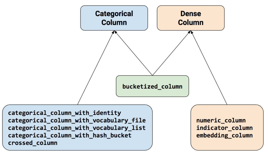
The rule of thumb is, at any time when you could have one thing categorical, together with crossed, it’s essential to then remodel it into one thing numeric, which incorporates indicator and embedding.
Being a heuristic, this rule works total, and it matches our instinct. There’s one exception although, step_bucketized_column, which though it “feels” categorical really doesn’t want that conversion.
Due to this fact, it’s best to complement that instinct with a easy lookup diagram, which can be a part of the feature columns vignette.
With this diagram, the easy rule is: We at all times want to finish up with one thing that inherits from DenseColumn. So:
step_numeric_column,step_indicator_column, andstep_embedding_columnare standalone;step_bucketized_columnis, too, nevertheless categorical it “feels”; and- all
step_categorical_column_[...], in addition tostep_crossed_column, have to be reworked utilizing one the dense column sorts.

Determine 1: To be used with Keras, all options want to finish up inheriting from DenseColumn someway.
Thus, we are able to repair the state of affairs like so:
and now ft_spec$dense_features() will present us
$rugged
NumericColumn(key='rugged', form=(1,), default_value=None, dtype=tf.float32, normalizer_fn=None)

$indicator_africa
IndicatorColumn(categorical_column=IdentityCategoricalColumn(key='africa', number_buckets=2.0, default_value=None))
What we actually wished to do is seize the interplay between ruggedness and continent. To this finish, we first bucketize rugged, after which cross it with – already binary – africa. As per the foundations, we lastly remodel into an indicator column:
ft_spec <- coaching %>%
  feature_spec(log_gdp ~ .) %>%
  step_numeric_column(rugged) %>%
  step_categorical_column_with_identity(africa, num_buckets = 2) %>%
  step_indicator_column(africa) %>%
  step_bucketized_column(rugged,
                         boundaries = c(0.1, 0.2, 0.3, 0.4, 0.5, 0.6, 0.8)) %>%
  step_crossed_column(africa_rugged_interact = c(africa, bucketized_rugged),
                      hash_bucket_size = 16) %>%
  step_indicator_column(africa_rugged_interact) %>%
  match()
Taking a look at this code you could be asking your self, now what number of options do I’ve within the mannequin?
Let’s verify.
$rugged
NumericColumn(key='rugged', form=(1,), default_value=None, dtype=tf.float32, normalizer_fn=None)

$indicator_africa
IndicatorColumn(categorical_column=IdentityCategoricalColumn(key='africa', number_buckets=2.0, default_value=None))

$bucketized_rugged
BucketizedColumn(source_column=NumericColumn(key='rugged', form=(1,), default_value=None, dtype=tf.float32, normalizer_fn=None), boundaries=(0.1, 0.2, 0.3, 0.4, 0.5, 0.6, 0.8))

$indicator_africa_rugged_interact
IndicatorColumn(categorical_column=CrossedColumn(keys=(IdentityCategoricalColumn(key='africa', number_buckets=2.0, default_value=None), BucketizedColumn(source_column=NumericColumn(key='rugged', form=(1,), default_value=None, dtype=tf.float32, normalizer_fn=None), boundaries=(0.1, 0.2, 0.3, 0.4, 0.5, 0.6, 0.8))), hash_bucket_size=16.0, hash_key=None))
We see that every one options, unique or reworked, are stored, so long as they inherit from DenseColumn.
Which means, for instance, the non-bucketized, steady values of rugged are used as properly.
Now organising the coaching goes as anticipated.
inputs <- layer_input_from_dataset(df %>% select(-log_gdp))

output <- inputs %>%
  layer_dense_features(ft_spec$dense_features()) %>%
  layer_dense(items = 8, activation = "relu") %>%
  layer_dense(items = 8, activation = "relu") %>%
  layer_dense(items = 1)

mannequin <- keras_model(inputs, output)

mannequin %>% compile(loss = "mse", optimizer = "adam", metrics = "mse")

historical past <- mannequin %>% match(
  x = coaching,
  y = coaching$log_gdp,
  validation_data = list(testing, testing$log_gdp),
  epochs = 100)
Simply as a sanity verify, the ultimate loss on the validation set for this code was ~ 0.014. However actually this instance did serve completely different functions.
In a nutshell
Characteristic specs are a handy, elegant method of creating categorical knowledge out there to Keras, in addition to to chain helpful transformations like bucketizing and creating crossed columns. The time you save knowledge wrangling could go into tuning and experimentation. Take pleasure in, and thanks for studying!
Yan, Lian, Robert H Dodier, Michael Mozer, and Richard H Wolniewicz. 2003. “Optimizing Classifier Efficiency by way of an Approximation to the Wilcoxon-Mann-Whitney Statistic.” In Proceedings of the twentieth Worldwide Convention on Machine Studying (ICML-03), 848–55.


