A really first conceptual introduction to Hamiltonian Monte Carlo

Why a very (that means: VERY!) first conceptual introduction to Hamiltonian Monte Carlo (HMC) on this weblog?

Nicely, in our endeavor to function the assorted capabilities of TensorFlow Likelihood (TFP) / tfprobability, we began displaying examples of the way to match hierarchical fashions, utilizing considered one of TFP’s joint distribution lessons and HMC. The technical features being complicated sufficient in themselves, we by no means gave an introduction to the “math facet of issues.” Right here we are attempting to make up for this.

Seeing how it’s unimaginable, in a brief weblog submit, to offer an introduction to Bayesian modeling and Markov Chain Monte Carlo on the whole, and the way there are such a lot of wonderful texts doing this already, we are going to presuppose some prior data. Our particular focus then is on the most recent and biggest, the magic buzzwords, the well-known incantations: Hamiltonian Monte Carlo, leapfrog steps, NUTS – as all the time, making an attempt to demystify, to make issues as comprehensible as potential.
In that spirit, welcome to a “glossary with a story.”

So what’s it for?

Sampling, or Monte Carlo, methods on the whole are used after we wish to produce samples from, or statistically describe a distribution we don’t have a closed-form formulation of. Typically, we would actually have an interest within the samples; typically we simply need them so we will compute, for instance, the imply and variance of the distribution.

What distribution? In the kind of functions we’re speaking about, we have now a mannequin, a joint distribution, which is meant to explain some actuality. Ranging from probably the most primary state of affairs, it would seem like this:

[
x sim mathcal{Poisson}(lambda)
]

This “joint distribution” solely has a single member, a Poisson distribution, that’s purported to mannequin, say, the variety of feedback in a code overview. We even have information on precise code critiques, like this, say:

We now wish to decide the parameter, (lambda), of the Poisson that make these information most seemingly. To date, we’re not even being Bayesian but: There is no such thing as a prior on this parameter. However after all, we wish to be Bayesian, so we add one – think about mounted priors on its parameters:

[
x sim mathcal{Poisson}(lambda)
lambda sim gamma(alpha, beta)
alpha sim […]
beta sim […]
]

This being a joint distribution, we have now three parameters to find out: (lambda), (alpha) and (beta).
And what we’re all in favour of is the posterior distribution of the parameters given the info.

Now, relying on the distributions concerned, we often can’t calculate the posterior distributions in closed kind. As a substitute, we have now to make use of sampling methods to find out these parameters. What we’d prefer to level out as an alternative is the next: Within the upcoming discussions of sampling, HMC & co., it’s very easy to overlook what’s it that we’re sampling. Attempt to all the time remember the fact that what we’re sampling isn’t the info, it’s parameters: the parameters of the posterior distributions we’re all in favour of.

Sampling

Sampling strategies on the whole include two steps: producing a pattern (“proposal”) and deciding whether or not to maintain it or to throw it away (“acceptance”). Intuitively, in our given state of affairs – the place we have now measured one thing and at the moment are in search of a mechanism that explains these measurements – the latter needs to be simpler: We “simply” want to find out the probability of the info beneath these hypothetical mannequin parameters. However how will we give you solutions to begin with?

In principle, easy(-ish) strategies exist that could possibly be used to generate samples from an unknown (in closed kind) distribution – so long as their unnormalized chances will be evaluated, and the issue is (very) low-dimensional. (For concise portraits of these strategies, comparable to uniform sampling, significance sampling, and rejection sampling, see(MacKay 2002).) These should not utilized in MCMC software program although, for lack of effectivity and non-suitability in excessive dimensions. Earlier than HMC grew to become the dominant algorithm in such software program, the Metropolis and Gibbs strategies had been the algorithms of alternative. Each are properly and understandably defined – within the case of Metropolis, usually exemplified by good tales –, and we refer the reader to the go-to references, comparable to (McElreath 2016) and (Kruschke 2010). Each had been proven to be much less environment friendly than HMC, the primary subject of this submit, as a result of their random-walk habits: Each proposal relies on the present place in state house, that means that samples could also be extremely correlated and state house exploration proceeds slowly.

HMC

So HMC is widespread as a result of in comparison with random-walk-based algorithms, it’s a lot extra environment friendly. Sadly, it’s also much more tough to “get.” As mentioned in Math, code, concepts: A third road to deep learning, there appear to be (at the least) three languages to specific an algorithm: Math; code (together with pseudo-code, which can or is probably not on the verge to math notation); and one I name conceptual which spans the entire vary from very summary to very concrete, even visible. To me personally, HMC is completely different from most different circumstances in that although I discover the conceptual explanations fascinating, they lead to much less “perceived understanding” than both the equations or the code. For individuals with backgrounds in physics, statistical mechanics and/or differential geometry this can in all probability be completely different!

In any case, bodily analogies make for the perfect begin.

Bodily analogies

The traditional bodily analogy is given within the reference article, Radford Neal’s “MCMC utilizing Hamiltonian dynamics” (Neal 2012), and properly defined in a video by Ben Lambert.

So there’s this “factor” we wish to maximize, the loglikelihood of the info beneath the mannequin parameters. Alternatively we will say, we wish to decrease the detrimental loglikelihood (like loss in a neural community). This “factor” to be optimized can then be visualized as an object sliding over a panorama with hills and valleys, and like with gradient descent in deep studying, we would like it to finish up deep down in some valley.

In Neal’s personal phrases

In two dimensions, we will visualize the dynamics as that of a frictionless puck that slides over a floor of various top. The state of this method consists of the place of the puck, given by a 2D vector q, and the momentum of the puck (its mass instances its velocity), given by a 2D vector p.

Now while you hear “momentum” (and provided that I’ve primed you to think about deep studying) you might really feel that sounds acquainted, however although the respective analogies are associated the affiliation doesn’t assist that a lot. In deep studying, momentum is often praised for its avoidance of ineffective oscillations in imbalanced optimization landscapes.
With HMC nevertheless, the main target is on the idea of power.

In statistical mechanics, the chance of being in some state (i) is inverse-exponentially associated to its power. (Right here (T) is the temperature; we received’t give attention to this so simply think about it being set to 1 on this and subsequent equations.)

[P(E_i) sim e^{frac{-E_i}{T}} ]

As you may or won’t keep in mind from faculty physics, power is available in two kinds: potential power and kinetic power. Within the sliding-object state of affairs, the thing’s potential power corresponds to its top (place), whereas its kinetic power is said to its momentum, (m), by the components

[K(m) = frac{m^2}{2 * mass} ]

Now with out kinetic power, the thing would slide downhill all the time, and as quickly because the panorama slopes up once more, would come to a halt. By way of its momentum although, it is ready to proceed uphill for some time, simply as if, going downhill in your bike, you decide up pace you might make it over the following (quick) hill with out pedaling.

In order that’s kinetic power. The opposite half, potential power, corresponds to the factor we actually wish to know – the detrimental log posterior of the parameters we’re actually after:

[U(theta) sim – log (P(x | theta) P(theta))]

So the “trick” of HMC is augmenting the state house of curiosity – the vector of posterior parameters – by a momentum vector, to enhance optimization effectivity. After we’re completed, the momentum half is simply thrown away. (This facet is very properly defined in Ben Lambert’s video.)

Following his exposition and notation, right here we have now the power of a state of parameter and momentum vectors, equaling a sum of potential and kinetic energies:

[E(theta, m) = U(theta) + K(m)]

The corresponding chance, as per the connection given above, then is

[P(E) sim e^{frac{-E}{T}} = e^{frac{- U(theta)}{T}} e^{frac{- K(m)}{T}}]

We now substitute into this equation, assuming a temperature (T) of 1 and a mass of 1:

[P(E) sim P(x | theta) P(theta) e^{frac{- m^2}{2}}]

Now on this formulation, the distribution of momentum is simply a regular regular ((e^{frac{- m^2}{2}}))! Thus, we will simply combine out the momentum and take (P(theta)) as samples from the posterior distribution:

[
begin{aligned}
& P(theta) =
int ! P(theta, m) mathrm{d}m = frac{1}{Z} int ! P(x | theta) P(theta) mathcal{N}(m|0,1) mathrm{d}m
& P(theta) = frac{1}{Z} int ! P(x | theta) P(theta)
end{aligned}
]

How does this work in observe? At each step, we

• pattern a brand new momentum worth from its marginal distribution (which is similar because the conditional distribution given (U), as they’re unbiased), and
• resolve for the trail of the particle. That is the place Hamilton’s equations come into play.

Hamilton’s equations (equations of movement)

For the sake of much less confusion, do you have to resolve to learn the paper, right here we change to Radford Neal’s notation.

Hamiltonian dynamics operates on a d-dimensional place vector, (q), and a d-dimensional momentum vector, (p). The state house is described by the Hamiltonian, a perform of (p) and (q):

[H(q, p) =U(q) +K(p)]

Right here (U(q)) is the potential power (referred to as (U(theta)) above), and (Ok(p)) is the kinetic power as a perform of momentum (referred to as (Ok(m)) above).

The partial derivatives of the Hamiltonian decide how (p) and (q) change over time, (t), in response to Hamilton’s equations:

[
begin{aligned}
& frac{dq}{dt} = frac{partial H}{partial p}
& frac{dp}{dt} = – frac{partial H}{partial q}
end{aligned}
]

How can we resolve this method of partial differential equations? The fundamental workhorse in numerical integration is Euler’s technique, the place time (or the unbiased variable, on the whole) is superior by a step of measurement (epsilon), and a brand new worth of the dependent variable is computed by taking the (partial) spinoff and including it to its present worth. For the Hamiltonian system, doing this one equation after the opposite appears to be like like this:

[
begin{aligned}
& p(t+epsilon) = p(t) + epsilon frac{dp}{dt}(t) = p(t) − epsilon frac{partial U}{partial q}(q(t))
& q(t+epsilon) = q(t) + epsilon frac{dq}{dt}(t) = q(t) + epsilon frac{p(t)}{m})
end{aligned}
]

Right here first a brand new place is computed for time (t + 1), making use of the present momentum at time (t); then a brand new momentum is computed, additionally for time (t + 1), making use of the present place at time (t).

This course of will be improved if in step 2, we make use of the new place we simply freshly computed in step 1; however let’s immediately go to what’s truly utilized in modern software program, the leapfrog technique.

Leapfrog algorithm

So after Hamiltonian, we’ve hit the second magic phrase: leapfrog. In contrast to Hamiltonian nevertheless, there may be much less thriller right here. The leapfrog technique is “simply” a extra environment friendly method to carry out the numerical integration.

It consists of three steps, principally splitting up the Euler step 1 into two components, earlier than and after the momentum replace:

[
begin{aligned}
& p(t+frac{epsilon}{2}) = p(t) − frac{epsilon}{2} frac{partial U}{partial q}(q(t))
& q(t+epsilon) = q(t) + epsilon frac{p(t + frac{epsilon}{2})}{m}
& p(t+ epsilon) = p(t+frac{epsilon}{2}) − frac{epsilon}{2} frac{partial U}{partial q}(q(t + epsilon))
end{aligned}
]

As you possibly can see, every step makes use of the corresponding variable-to-differentiate’s worth computed within the previous step. In observe, a number of leapfrog steps are executed earlier than a proposal is made; so steps 3 and 1 (of the following iteration) are mixed.

Proposal – this key phrase brings us again to the higher-level “plan.” All this – Hamiltonian equations, leapfrog integration – served to generate a proposal for a brand new worth of the parameters, which will be accepted or not. The way in which that call is taken will not be specific to HMC and defined intimately within the above-mentioned expositions on the Metropolis algorithm, so we simply cowl it briefly.

Acceptance: Metropolis algorithm

Below the Metropolis algorithm, proposed new vectors (q*) and (p*) are accepted with chance

[
min(1, exp(−H(q∗, p∗) +H(q, p)))
]

That’s, if the proposed parameters yield a better probability, they’re accepted; if not, they’re accepted solely with a sure chance that is dependent upon the ratio between outdated and new likelihoods.
In principle, power staying fixed in a Hamiltonian system, proposals ought to all the time be accepted; in observe, lack of precision as a result of numerical integration might yield an acceptance fee lower than 1.

HMC in just a few strains of code

We’ve talked about ideas, and we’ve seen the mathematics, however between analogies and equations, it’s simple to lose monitor of the general algorithm. Properly, Radford Neal’s paper (Neal 2012) has some code, too! Right here it’s reproduced, with just some further feedback added (many feedback had been preexisting):

# U is a perform that returns the potential power given q
# grad_U returns the respective partial derivatives
# epsilon stepsize
# L variety of leapfrog steps
# current_q present place

# kinetic power is assumed to be sum(p^2/2) (mass == 1)
HMC <- perform (U, grad_U, epsilon, L, current_q) {
  q <- current_q
  # unbiased commonplace regular variates
  p <- rnorm(length(q), 0, 1)  
  # Make a half step for momentum in the beginning
  current_p <- p 
  # Alternate full steps for place and momentum
  p <- p - epsilon * grad_U(q) / 2 
  for (i in 1:L) {
    # Make a full step for the place
    q <- q + epsilon * p
    # Make a full step for the momentum, besides at finish of trajectory
    if (i != L) p <- p - epsilon * grad_U(q)
    }
  # Make a half step for momentum on the finish
  p <- p - epsilon * grad_U(q) / 2
  # Negate momentum at finish of trajectory to make the proposal symmetric
  p <- -p
  # Consider potential and kinetic energies at begin and finish of trajectory 
  current_U <- U(current_q)
  current_K <- sum(current_p^2) / 2
  proposed_U <- U(q)
  proposed_K <- sum(p^2) / 2
  # Settle for or reject the state at finish of trajectory, returning both
  # the place on the finish of the trajectory or the preliminary place
  if (runif(1) < exp(current_U-proposed_U+current_K-proposed_K)) {
    return (q)  # settle for
  } else {
    return (current_q)  # reject
  }
}

Hopefully, you discover this piece of code as useful as I do. Are we by but? Nicely, to this point we haven’t encountered the final magic phrase: NUTS. What, or who, is NUTS?

NUTS

NUTS, added to Stan in 2011 and a few month in the past, to TensorFlow Probability’s master branch, is an algorithm that goals to bypass one of many sensible difficulties in utilizing HMC: The selection of variety of leapfrog steps to carry out earlier than making a proposal. The acronym stands for No-U-Flip Sampler, alluding to the avoidance of U-turn-shaped curves within the optimization panorama when the variety of leapfrog steps is chosen too excessive.

The reference paper by Hoffman & Gelman (Hoffman and Gelman 2011) additionally describes an answer to a associated issue: selecting the step measurement (epsilon). The respective algorithm, twin averaging, was also recently added to TFP.

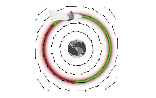
NUTS being extra of algorithm within the laptop science utilization of the phrase than a factor to elucidate conceptually, we’ll depart it at that, and ask the reader to learn the paper – and even, consult the TFP documentation to see how NUTS is implemented there. As a substitute, we’ll spherical up with one other conceptual analogy, Michael Bétancourts crashing (or not!) satellite tv for pc (Betancourt 2017).

The right way to keep away from crashes

Bétancourt’s article is an superior learn, and a paragraph specializing in a single level made within the paper will be nothing than a “teaser” (which is why we’ll have an image, too!).

To introduce the upcoming analogy, the issue begins with excessive dimensionality, which is a given in most real-world issues. In excessive dimensions, as common, the density perform has a mode (the place the place it’s maximal), however essentially, there can’t be a lot quantity round it – similar to with k-nearest neighbors, the extra dimensions you add, the farther your nearest neighbor will likely be.
A product of quantity and density, the one important chance mass resides within the so-called typical set, which turns into increasingly more slim in excessive dimensions.

So, the standard set is what we wish to discover, but it surely will get increasingly more tough to search out it (and keep there). Now as we noticed above, HMC makes use of gradient data to get close to the mode, but when it simply adopted the gradient of the log chance (the place) it could depart the standard set and cease on the mode.

That is the place momentum is available in – it counteracts the gradient, and each collectively be sure that the Markov chain stays on the standard set. Now right here’s the satellite tv for pc analogy, in Bétancourt’s personal phrases:

For instance, as an alternative of making an attempt to cause a few mode, a gradient, and a typical set, we will equivalently cause a few planet, a gravitational discipline, and an orbit (Determine 14). The probabilistic endeavor of exploring the standard set then turns into a bodily endeavor of putting a satellite tv for pc in a steady orbit across the hypothetical planet. As a result of these are simply two completely different views of the identical mathematical system, they’ll undergo from the identical pathologies. Certainly, if we place a satellite tv for pc at relaxation out in house it is going to fall within the gravitational discipline and crash into the floor of the planet, simply as naive gradient-driven trajectories crash into the mode (Determine 15). From both the probabilistic or bodily perspective we’re left with a catastrophic consequence.

The bodily image, nevertheless, gives a right away answer: though objects at relaxation will crash into the planet, we will preserve a steady orbit by endowing our satellite tv for pc with sufficient momentum to counteract the gravitational attraction. We’ve got to watch out, nevertheless, in how precisely we add momentum to our satellite tv for pc. If we add too little momentum transverse to the gravitational discipline, for instance, then the gravitational attraction will likely be too sturdy and the satellite tv for pc will nonetheless crash into the planet (Determine 16a). However, if we add an excessive amount of momentum then the gravitational attraction will likely be too weak to seize the satellite tv for pc in any respect and it’ll as an alternative fly out into the depths of house (Determine 16b).

And right here’s the image I promised (Determine 16 from the paper):

And with this, we conclude. Hopefully, you’ll have discovered this useful – except you knew all of it (or extra) beforehand, by which case you in all probability wouldn’t have learn this submit 🙂

Thanks for studying!