Posit AI Weblog: Variational convnets with tfprobability

A bit greater than a yr in the past, in his lovely guest post, Nick Strayer confirmed methods to classify a set of on a regular basis actions utilizing smartphone-recorded gyroscope and accelerometer information. Accuracy was superb, however Nick went on to examine classification outcomes extra carefully. Have been there actions extra liable to misclassification than others? And the way about these faulty outcomes: Did the community report them with equal, or much less confidence than people who have been appropriate?

Technically, after we communicate of confidence in that method, we’re referring to the rating obtained for the “profitable” class after softmax activation. If that profitable rating is 0.9, we’d say “the community is bound that’s a gentoo penguin”; if it’s 0.2, we’d as a substitute conclude “to the community, neither choice appeared becoming, however cheetah seemed greatest.”

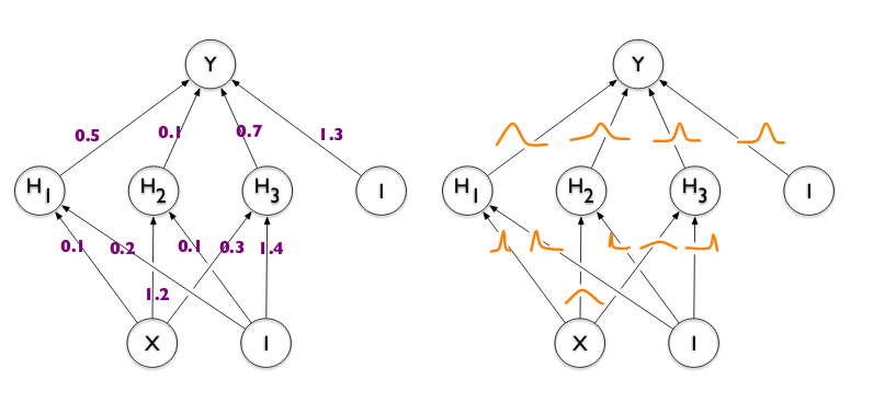
This use of “confidence” is convincing, nevertheless it has nothing to do with confidence – or credibility, or prediction, what have you ever – intervals. What we’d actually like to have the ability to do is put distributions over the community’s weights and make it Bayesian. Utilizing tfprobability’s variational Keras-compatible layers, that is one thing we really can do.

Adding uncertainty estimates to Keras models with tfprobability exhibits methods to use a variational dense layer to acquire estimates of epistemic uncertainty. On this put up, we modify the convnet utilized in Nick’s put up to be variational all through. Earlier than we begin, let’s rapidly summarize the duty.

The duty

To create the Smartphone-Based Recognition of Human Activities and Postural Transitions Data Set (Reyes-Ortiz et al. 2016), the researchers had topics stroll, sit, stand, and transition from a kind of actions to a different. In the meantime, two forms of smartphone sensors have been used to document movement information: Accelerometers measure linear acceleration in three dimensions, whereas gyroscopes are used to trace angular velocity across the coordinate axes. Listed below are the respective uncooked sensor information for six forms of actions from Nick’s unique put up:

Identical to Nick, we’re going to zoom in on these six forms of exercise, and attempt to infer them from the sensor information. Some information wrangling is required to get the dataset right into a type we are able to work with; right here we’ll construct on Nick’s put up, and successfully begin from the info properly pre-processed and cut up up into coaching and take a look at units:

Observations: 289
Variables: 6
$ experiment    <int> 1, 2, 3, 4, 5, 6, 7, 8, 9, 10, 13, 14, 17, 18, 19, 2…
$ userId        <int> 1, 1, 2, 2, 3, 3, 4, 4, 5, 5, 7, 7, 9, 9, 10, 10, 11…
$ exercise      <int> 7, 7, 7, 7, 7, 7, 7, 7, 7, 7, 7, 7, 7, 7, 7, 7, 7, 7…
$ information          <checklist> [<data.frame[160 x 6]>, <information.body[206 x 6]>, <dat…
$ activityName  <fct> STAND_TO_SIT, STAND_TO_SIT, STAND_TO_SIT, STAND_TO_S…
$ observationId <int> 1, 2, 3, 4, 5, 6, 7, 8, 9, 10, 13, 14, 17, 18, 19, 2…

Observations: 69
Variables: 6
$ experiment    <int> 11, 12, 15, 16, 32, 33, 42, 43, 52, 53, 56, 57, 11, …
$ userId        <int> 6, 6, 8, 8, 16, 16, 21, 21, 26, 26, 28, 28, 6, 6, 8,…
$ exercise      <int> 7, 7, 7, 7, 7, 7, 7, 7, 7, 7, 7, 7, 8, 8, 8, 8, 8, 8…
$ information          <checklist> [<data.frame[185 x 6]>, <information.body[151 x 6]>, <dat…
$ activityName  <fct> STAND_TO_SIT, STAND_TO_SIT, STAND_TO_SIT, STAND_TO_S…
$ observationId <int> 11, 12, 15, 16, 31, 32, 41, 42, 51, 52, 55, 56, 71, …

The code required to reach at this stage (copied from Nick’s put up) could also be discovered within the appendix on the backside of this web page.

Coaching pipeline

The dataset in query is sufficiently small to slot in reminiscence – however yours won’t be, so it could’t damage to see some streaming in motion. Apart from, it’s most likely protected to say that with TensorFlow 2.0, tfdatasets pipelines are the option to feed information to a mannequin.

As soon as the code listed within the appendix has run, the sensor information is to be present in trainData$information, a listing column containing information.bodys the place every row corresponds to some extent in time and every column holds one of many measurements. Nonetheless, not all time collection (recordings) are of the identical size; we thus observe the unique put up to pad all collection to size pad_size (= 338). The anticipated form of coaching batches will then be (batch_size, pad_size, 6).

We initially create our coaching dataset:

train_x <- train_data$information %>% 
  map(as.matrix) %>%
  pad_sequences(maxlen = pad_size, dtype = "float32") %>%
  tensor_slices_dataset() 

train_y <- train_data$exercise %>% 
  one_hot_classes() %>% 
  tensor_slices_dataset()

train_dataset <- zip_datasets(train_x, train_y)
train_dataset

<ZipDataset shapes: ((338, 6), (6,)), sorts: (tf.float64, tf.float64)>

Then shuffle and batch it:

n_train <- nrow(train_data)
# the best attainable batch measurement for this dataset
# chosen as a result of it yielded one of the best efficiency
# alternatively, experiment with e.g. totally different studying charges, ...
batch_size <- n_train

train_dataset <- train_dataset %>% 
  dataset_shuffle(n_train) %>%
  dataset_batch(batch_size)
train_dataset

<BatchDataset shapes: ((None, 338, 6), (None, 6)), sorts: (tf.float64, tf.float64)>

Identical for the take a look at information.

test_x <- test_data$information %>% 
  map(as.matrix) %>%
  pad_sequences(maxlen = pad_size, dtype = "float32") %>%
  tensor_slices_dataset() 

test_y <- test_data$exercise %>% 
  one_hot_classes() %>% 
  tensor_slices_dataset()

n_test <- nrow(test_data)
test_dataset <- zip_datasets(test_x, test_y) %>%
  dataset_batch(n_test)

Utilizing tfdatasets doesn’t imply we can not run a fast sanity verify on our information:

first <- test_dataset %>% 
  reticulate::as_iterator() %>% 
  # get first batch (= entire take a look at set, in our case)
  reticulate::iter_next() %>%
  # predictors solely
  .[[1]] %>% 
  # first merchandise in batch
  .[1,,]
first

tf.Tensor(
[[ 0.          0.          0.          0.          0.          0.        ]
 [ 0.          0.          0.          0.          0.          0.        ]
 [ 0.          0.          0.          0.          0.          0.        ]
 ...
 [ 1.00416672  0.2375      0.12916666 -0.40225476 -0.20463985 -0.14782938]
 [ 1.04166663  0.26944447  0.12777779 -0.26755899 -0.02779437 -0.1441642 ]
 [ 1.0250001   0.27083334  0.15277778 -0.19639318  0.35094208 -0.16249016]],
 form=(338, 6), dtype=float64)

Now let’s construct the community.

A variational convnet

We construct on the simple convolutional structure from Nick’s put up, simply making minor modifications to kernel sizes and numbers of filters. We additionally throw out all dropout layers; no extra regularization is required on high of the priors utilized to the weights.

Word the next concerning the “Bayesified” community.

• Every layer is variational in nature, the convolutional ones (layer_conv_1d_flipout) in addition to the dense layers (layer_dense_flipout).

• With variational layers, we are able to specify the prior weight distribution in addition to the type of the posterior; right here the defaults are used, leading to an ordinary regular prior and a default mean-field posterior.

• Likewise, the consumer could affect the divergence perform used to evaluate the mismatch between prior and posterior; on this case, we really take some motion: We scale the (default) KL divergence by the variety of samples within the coaching set.

• One very last thing to notice is the output layer. It’s a distribution layer, that’s, a layer wrapping a distribution – the place wrapping means: Coaching the community is enterprise as common, however predictions are distributions, one for every information level.

library(tfprobability)

num_classes <- 6

# scale the KL divergence by variety of coaching examples
n <- n_train %>% tf$forged(tf$float32)
kl_div <- perform(q, p, unused)
  tfd_kl_divergence(q, p) / n

mannequin <- keras_model_sequential()
mannequin %>% 
  layer_conv_1d_flipout(
    filters = 12,
    kernel_size = 3, 
    activation = "relu",
    kernel_divergence_fn = kl_div
  ) %>%
  layer_conv_1d_flipout(
    filters = 24,
    kernel_size = 5, 
    activation = "relu",
    kernel_divergence_fn = kl_div
  ) %>%
  layer_conv_1d_flipout(
    filters = 48,
    kernel_size = 7, 
    activation = "relu",
    kernel_divergence_fn = kl_div
  ) %>%
  layer_global_average_pooling_1d() %>% 
  layer_dense_flipout(
    items = 48,
    activation = "relu",
    kernel_divergence_fn = kl_div
  ) %>% 
  layer_dense_flipout(
    num_classes, 
    kernel_divergence_fn = kl_div,
    identify = "dense_output"
  ) %>%
  layer_one_hot_categorical(event_size = num_classes)

We inform the community to reduce the adverse log chance.

nll <- perform(y, mannequin) - (mannequin %>% tfd_log_prob(y))

This can turn out to be a part of the loss. The best way we arrange this instance, this isn’t its most substantial half although. Right here, what dominates the loss is the sum of the KL divergences, added (robotically) to mannequin$losses.

In a setup like this, it’s fascinating to observe each components of the loss individually. We will do that by way of two metrics:

# the KL a part of the loss
kl_part <-  perform(y_true, y_pred) {
    kl <- tf$reduce_sum(mannequin$losses)
    kl
}

# the NLL half
nll_part <- perform(y_true, y_pred) {
    cat_dist <- tfd_one_hot_categorical(logits = y_pred)
    nll <- - (cat_dist %>% tfd_log_prob(y_true) %>% tf$reduce_mean())
    nll
}

We prepare considerably longer than Nick did within the unique put up, permitting for early stopping although.

mannequin %>% compile(
  optimizer = "rmsprop",
  loss = nll,
  metrics = c("accuracy", 
              custom_metric("kl_part", kl_part),
              custom_metric("nll_part", nll_part)),
  experimental_run_tf_function = FALSE
)

train_history <- mannequin %>% match(
  train_dataset,
  epochs = 1000,
  validation_data = test_dataset,
  callbacks = list(
    callback_early_stopping(persistence = 10)
  )
)

Whereas the general loss declines linearly (and possibly would for a lot of extra epochs), this isn’t the case for classification accuracy or the NLL a part of the loss:

Closing accuracy just isn’t as excessive as within the non-variational setup, although nonetheless not unhealthy for a six-class downside. We see that with none extra regularization, there may be little or no overfitting to the coaching information.

Now how will we get hold of predictions from this mannequin?

Probabilistic predictions

Although we gained’t go into this right here, it’s good to know that we entry extra than simply the output distributions; by their kernel_posterior attribute, we are able to entry the hidden layers’ posterior weight distributions as nicely.

Given the small measurement of the take a look at set, we compute all predictions directly. The predictions are actually categorical distributions, one for every pattern within the batch:

test_data_all <- dataset_collect(test_dataset) %>% { .[[1]][[1]]}

one_shot_preds <- mannequin(test_data_all) 

one_shot_preds

tfp.distributions.OneHotCategorical(
 "sequential_one_hot_categorical_OneHotCategorical_OneHotCategorical",
 batch_shape=[69], event_shape=[6], dtype=float32)

We prefixed these predictions with one_shot to point their noisy nature: These are predictions obtained on a single cross by the community, all layer weights being sampled from their respective posteriors.

From the expected distributions, we calculate imply and normal deviation per (take a look at) pattern.

one_shot_means <- tfd_mean(one_shot_preds) %>% 
  as.matrix() %>%
  as_tibble() %>% 
  mutate(obs = 1:n()) %>% 
  collect(class, imply, -obs) 

one_shot_sds <- tfd_stddev(one_shot_preds) %>% 
  as.matrix() %>%
  as_tibble() %>% 
  mutate(obs = 1:n()) %>% 
  collect(class, sd, -obs) 

The usual deviations thus obtained may very well be mentioned to mirror the general predictive uncertainty. We will estimate one other form of uncertainty, known as epistemic, by making a lot of passes by the community after which, calculating – once more, per take a look at pattern – the usual deviations of the expected means.

mc_preds <- purrr::map(1:100, perform(x) {
  preds <- mannequin(test_data_all)
  tfd_mean(preds) %>% as.matrix()
})

mc_sds <- abind::abind(mc_preds, alongside = 3) %>% 
  apply(c(1,2), sd) %>% 
  as_tibble() %>%
  mutate(obs = 1:n()) %>% 
  collect(class, mc_sd, -obs) 

Placing all of it collectively, now we have

pred_data <- one_shot_means %>%
  inner_join(one_shot_sds, by = c("obs", "class")) %>% 
  inner_join(mc_sds, by = c("obs", "class")) %>% 
  right_join(one_hot_to_label, by = "class") %>% 
  organize(obs)

pred_data

# A tibble: 414 x 6
     obs class       imply      sd    mc_sd label       
   <int> <chr>      <dbl>   <dbl>    <dbl> <fct>       
 1     1 V1    0.945      0.227   0.0743   STAND_TO_SIT
 2     1 V2    0.0534     0.225   0.0675   SIT_TO_STAND
 3     1 V3    0.00114    0.0338  0.0346   SIT_TO_LIE  
 4     1 V4    0.00000238 0.00154 0.000336 LIE_TO_SIT  
 5     1 V5    0.0000132  0.00363 0.00164  STAND_TO_LIE
 6     1 V6    0.0000305  0.00553 0.00398  LIE_TO_STAND
 7     2 V1    0.993      0.0813  0.149    STAND_TO_SIT
 8     2 V2    0.00153    0.0390  0.102    SIT_TO_STAND
 9     2 V3    0.00476    0.0688  0.108    SIT_TO_LIE  
10     2 V4    0.00000172 0.00131 0.000613 LIE_TO_SIT  
# … with 404 extra rows

Evaluating predictions to the bottom fact:

eval_table <- pred_data %>% 
  group_by(obs) %>% 
  summarise(
    maxprob = max(imply),
    maxprob_sd = sd[mean == maxprob],
    maxprob_mc_sd = mc_sd[mean == maxprob],
    predicted = label[mean == maxprob]
  ) %>% 
  mutate(
    fact = test_data$activityName,
    appropriate = fact == predicted
  ) 

eval_table %>% print(n = 20)

# A tibble: 69 x 7
     obs maxprob maxprob_sd maxprob_mc_sd predicted    fact        appropriate
   <int>   <dbl>      <dbl>         <dbl> <fct>        <fct>        <lgl>  
 1     1   0.945     0.227         0.0743 STAND_TO_SIT STAND_TO_SIT TRUE   
 2     2   0.993     0.0813        0.149  STAND_TO_SIT STAND_TO_SIT TRUE   
 3     3   0.733     0.443         0.131  STAND_TO_SIT STAND_TO_SIT TRUE   
 4     4   0.796     0.403         0.138  STAND_TO_SIT STAND_TO_SIT TRUE   
 5     5   0.843     0.364         0.358  SIT_TO_STAND STAND_TO_SIT FALSE  
 6     6   0.816     0.387         0.176  SIT_TO_STAND STAND_TO_SIT FALSE  
 7     7   0.600     0.490         0.370  STAND_TO_SIT STAND_TO_SIT TRUE   
 8     8   0.941     0.236         0.0851 STAND_TO_SIT STAND_TO_SIT TRUE   
 9     9   0.853     0.355         0.274  SIT_TO_STAND STAND_TO_SIT FALSE  
10    10   0.961     0.195         0.195  STAND_TO_SIT STAND_TO_SIT TRUE   
11    11   0.918     0.275         0.168  STAND_TO_SIT STAND_TO_SIT TRUE   
12    12   0.957     0.203         0.150  STAND_TO_SIT STAND_TO_SIT TRUE   
13    13   0.987     0.114         0.188  SIT_TO_STAND SIT_TO_STAND TRUE   
14    14   0.974     0.160         0.248  SIT_TO_STAND SIT_TO_STAND TRUE   
15    15   0.996     0.0657        0.0534 SIT_TO_STAND SIT_TO_STAND TRUE   
16    16   0.886     0.318         0.0868 SIT_TO_STAND SIT_TO_STAND TRUE   
17    17   0.773     0.419         0.173  SIT_TO_STAND SIT_TO_STAND TRUE   
18    18   0.998     0.0444        0.222  SIT_TO_STAND SIT_TO_STAND TRUE   
19    19   0.885     0.319         0.161  SIT_TO_STAND SIT_TO_STAND TRUE   
20    20   0.930     0.255         0.271  SIT_TO_STAND SIT_TO_STAND TRUE   
# … with 49 extra rows

Are normal deviations larger for misclassifications?

eval_table %>% 
  group_by(fact, predicted) %>% 
  summarise(avg_mean = mean(maxprob),
            avg_sd = mean(maxprob_sd),
            avg_mc_sd = mean(maxprob_mc_sd)) %>% 
  mutate(appropriate = fact == predicted) %>%
  organize(avg_mc_sd) 

# A tibble: 2 x 5
  appropriate rely avg_mean avg_sd avg_mc_sd
  <lgl>   <int>    <dbl>  <dbl>     <dbl>
1 FALSE      19    0.775  0.380     0.237
2 TRUE       50    0.879  0.264     0.183

They’re; although maybe to not the extent we’d want.

With simply six courses, we are able to additionally examine normal deviations on the person prediction-target pairings degree.

eval_table %>% 
  group_by(fact, predicted) %>% 
  summarise(cnt = n(),
            avg_mean = mean(maxprob),
            avg_sd = mean(maxprob_sd),
            avg_mc_sd = mean(maxprob_mc_sd)) %>% 
  mutate(appropriate = fact == predicted) %>%
  organize(desc(cnt), avg_mc_sd) 

# A tibble: 14 x 7
# Teams:   fact [6]
   fact        predicted      cnt avg_mean avg_sd avg_mc_sd appropriate
   <fct>        <fct>        <int>    <dbl>  <dbl>     <dbl> <lgl>  
 1 SIT_TO_STAND SIT_TO_STAND    12    0.935  0.205    0.184  TRUE   
 2 STAND_TO_SIT STAND_TO_SIT     9    0.871  0.284    0.162  TRUE   
 3 LIE_TO_SIT   LIE_TO_SIT       9    0.765  0.377    0.216  TRUE   
 4 SIT_TO_LIE   SIT_TO_LIE       8    0.908  0.254    0.187  TRUE   
 5 STAND_TO_LIE STAND_TO_LIE     7    0.956  0.144    0.132  TRUE   
 6 LIE_TO_STAND LIE_TO_STAND     5    0.809  0.353    0.227  TRUE   
 7 SIT_TO_LIE   STAND_TO_LIE     4    0.685  0.436    0.233  FALSE  
 8 LIE_TO_STAND SIT_TO_STAND     4    0.909  0.271    0.282  FALSE  
 9 STAND_TO_LIE SIT_TO_LIE       3    0.852  0.337    0.238  FALSE  
10 STAND_TO_SIT SIT_TO_STAND     3    0.837  0.368    0.269  FALSE  
11 LIE_TO_STAND LIE_TO_SIT       2    0.689  0.454    0.233  FALSE  
12 LIE_TO_SIT   STAND_TO_SIT     1    0.548  0.498    0.0805 FALSE  
13 SIT_TO_STAND LIE_TO_STAND     1    0.530  0.499    0.134  FALSE  
14 LIE_TO_SIT   LIE_TO_STAND     1    0.824  0.381    0.231  FALSE  

Once more, we see larger normal deviations for fallacious predictions, however to not a excessive diploma.

Conclusion

We’ve proven methods to construct, prepare, and acquire predictions from a completely variational convnet. Evidently, there may be room for experimentation: Various layer implementations exist; a distinct prior may very well be specified; the divergence may very well be calculated otherwise; and the standard neural community hyperparameter tuning choices apply.

Then, there’s the query of penalties (or: determination making). What will occur in high-uncertainty instances, what even is a high-uncertainty case? Naturally, questions like these are out-of-scope for this put up, but of important significance in real-world purposes.
Thanks for studying!

Appendix

To be executed earlier than operating this put up’s code. Copied from Classifying physical activity from smartphone data.

library(keras)     
library(tidyverse) 

activity_labels <- read.table("information/activity_labels.txt", 
                             col.names = c("quantity", "label")) 

one_hot_to_label <- activity_labels %>% 
  mutate(quantity = quantity - 7) %>% 
  filter(quantity >= 0) %>% 
  mutate(class = paste0("V",quantity + 1)) %>% 
  choose(-quantity)

labels <- read.table(
  "information/RawData/labels.txt",
  col.names = c("experiment", "userId", "exercise", "startPos", "endPos")
)

dataFiles <- list.files("information/RawData")
dataFiles %>% head()

fileInfo <- data_frame(
  filePath = dataFiles
) %>%
  filter(filePath != "labels.txt") %>%
  separate(filePath, sep = '_',
           into = c("kind", "experiment", "userId"),
           take away = FALSE) %>%
  mutate(
    experiment = str_remove(experiment, "exp"),
    userId = str_remove_all(userId, "consumer|.txt")
  ) %>%
  unfold(kind, filePath)

# Learn contents of single file to a dataframe with accelerometer and gyro information.
readInData <- perform(experiment, userId){
  genFilePath = perform(kind) {
    paste0("information/RawData/", kind, "_exp",experiment, "_user", userId, ".txt")
  }
  bind_cols(
    read.table(genFilePath("acc"), col.names = c("a_x", "a_y", "a_z")),
    read.table(genFilePath("gyro"), col.names = c("g_x", "g_y", "g_z"))
  )
}

# Perform to learn a given file and get the observations contained alongside
# with their courses.
loadFileData <- perform(curExperiment, curUserId) {

  # load sensor information from file into dataframe
  allData <- readInData(curExperiment, curUserId)
  extractObservation <- perform(startPos, endPos){
    allData[startPos:endPos,]
  }

  # get statement areas on this file from labels dataframe
  dataLabels <- labels %>%
    filter(userId == as.integer(curUserId),
           experiment == as.integer(curExperiment))

  # extract observations as dataframes and save as a column in dataframe.
  dataLabels %>%
    mutate(
      information = map2(startPos, endPos, extractObservation)
    ) %>%
    choose(-startPos, -endPos)
}

# scan by all experiment and userId combos and collect information right into a dataframe.
allObservations <- map2_df(fileInfo$experiment, fileInfo$userId, loadFileData) %>%
  right_join(activityLabels, by = c("exercise" = "quantity")) %>%
  rename(activityName = label)

write_rds(allObservations, "allObservations.rds")

allObservations <- readRDS("allObservations.rds")

desiredActivities <- c(
  "STAND_TO_SIT", "SIT_TO_STAND", "SIT_TO_LIE", 
  "LIE_TO_SIT", "STAND_TO_LIE", "LIE_TO_STAND"  
)

filteredObservations <- allObservations %>% 
  filter(activityName %in% desiredActivities) %>% 
  mutate(observationId = 1:n())

# get all customers
userIds <- allObservations$userId %>% unique()

# randomly select 24 (80% of 30 people) for coaching
set.seed(42) # seed for reproducibility
trainIds <- sample(userIds, measurement = 24)

# set the remainder of the customers to the testing set
testIds <- setdiff(userIds,trainIds)

# filter information. 
# notice S.Ok.: renamed to train_data for consistency with 
# variable naming used on this put up
train_data <- filteredObservations %>% 
  filter(userId %in% trainIds)

# notice S.Ok.: renamed to test_data for consistency with 
# variable naming used on this put up
test_data <- filteredObservations %>% 
  filter(userId %in% testIds)

# notice S.Ok.: renamed to pad_size for consistency with 
# variable naming used on this put up
pad_size <- trainData$information %>% 
  map_int(nrow) %>% 
  quantile(p = 0.98) %>% 
  ceiling()

# notice S.Ok.: renamed to one_hot_classes for consistency with 
# variable naming used on this put up
one_hot_classes <- . %>% 
  {. - 7} %>%        # deliver integers right down to 0-6 from 7-12
  to_categorical()   # One-hot encode