Time sequence prediction with FNN-LSTM

At the moment, we decide up on the plan alluded to within the conclusion of the latest Deep attractors: Where deep learning meets
chaos: make use of that very same approach to generate forecasts for
empirical time sequence knowledge.

“That very same approach,” which for conciseness, I’ll take the freedom of referring to as FNN-LSTM, is because of William Gilpin’s
2020 paper “Deep reconstruction of unusual attractors from time sequence” (Gilpin 2020).

In a nutshell, the issue addressed is as follows: A system, recognized or assumed to be nonlinear and extremely depending on
preliminary situations, is noticed, leading to a scalar sequence of measurements. The measurements aren’t simply – inevitably –
noisy, however as well as, they’re – at greatest – a projection of a multidimensional state area onto a line.

Classically in nonlinear time sequence evaluation, such scalar sequence of observations are augmented by supplementing, at each
time limit, delayed measurements of that very same sequence – a way known as delay coordinate embedding (Sauer, Yorke, and Casdagli 1991). For
instance, as a substitute of only a single vector X1, we might have a matrix of vectors X1, X2, and X3, with X2 containing
the identical values as X1, however ranging from the third remark, and X3, from the fifth. On this case, the delay can be
2, and the embedding dimension, 3. Varied theorems state that if these
parameters are chosen adequately, it’s doable to reconstruct the entire state area. There’s a downside although: The
theorems assume that the dimensionality of the true state area is thought, which in lots of real-world purposes, gained’t be the
case.

That is the place Gilpin’s thought is available in: Prepare an autoencoder, whose intermediate illustration encapsulates the system’s
attractor. Not simply any MSE-optimized autoencoder although. The latent illustration is regularized by false nearest
neighbors (FNN) loss, a way generally used with delay coordinate embedding to find out an enough embedding dimension.
False neighbors are those that are shut in n-dimensional area, however considerably farther aside in n+1-dimensional area.
Within the aforementioned introductory post, we confirmed how this
approach allowed to reconstruct the attractor of the (artificial) Lorenz system. Now, we wish to transfer on to prediction.

We first describe the setup, together with mannequin definitions, coaching procedures, and knowledge preparation. Then, we let you know the way it
went.

Setup

From reconstruction to forecasting, and branching out into the true world

Within the earlier publish, we skilled an LSTM autoencoder to generate a compressed code, representing the attractor of the system.
As typical with autoencoders, the goal when coaching is similar because the enter, that means that total loss consisted of two
parts: The FNN loss, computed on the latent illustration solely, and the mean-squared-error loss between enter and
output. Now for prediction, the goal consists of future values, as many as we want to predict. Put otherwise: The
structure stays the identical, however as a substitute of reconstruction we carry out prediction, in the usual RNN approach. The place the standard RNN
setup would simply instantly chain the specified variety of LSTMs, we’ve got an LSTM encoder that outputs a (timestep-less) latent
code, and an LSTM decoder that ranging from that code, repeated as many instances as required, forecasts the required variety of
future values.

This after all implies that to judge forecast efficiency, we have to examine in opposition to an LSTM-only setup. That is precisely
what we’ll do, and comparability will become fascinating not simply quantitatively, however qualitatively as properly.

We carry out these comparisons on the 4 datasets Gilpin selected to display attractor reconstruction on observational
data. Whereas all of those, as is obvious from the pictures
in that pocket book, exhibit good attractors, we’ll see that not all of them are equally suited to forecasting utilizing easy
RNN-based architectures – with or with out FNN regularization. However even people who clearly demand a special method enable
for fascinating observations as to the impression of FNN loss.

Mannequin definitions and coaching setup

In all 4 experiments, we use the identical mannequin definitions and coaching procedures, the one differing parameter being the
variety of timesteps used within the LSTMs (for causes that may grow to be evident once we introduce the person datasets).

Each architectures had been chosen to be simple, and about comparable in variety of parameters – each principally consist
of two LSTMs with 32 models (n_recurrent will probably be set to 32 for all experiments).

FNN-LSTM

FNN-LSTM seems to be practically like within the earlier publish, aside from the truth that we cut up up the encoder LSTM into two, to uncouple
capability (n_recurrent) from maximal latent state dimensionality (n_latent, stored at 10 identical to earlier than).

# DL-related packages
library(tensorflow)
library(keras)
library(tfdatasets)
library(tfautograph)
library(reticulate)

# going to want these later
library(tidyverse)
library(cowplot)

encoder_model <- perform(n_timesteps,
                          n_features,
                          n_recurrent,
                          n_latent,
                          title = NULL) {
  
  keras_model_custom(title = title, perform(self) {
    
    self$noise <- layer_gaussian_noise(stddev = 0.5)
    self$lstm1 <-  layer_lstm(
      models = n_recurrent,
      input_shape = c(n_timesteps, n_features),
      return_sequences = TRUE
    ) 
    self$batchnorm1 <- layer_batch_normalization()
    self$lstm2 <-  layer_lstm(
      models = n_latent,
      return_sequences = FALSE
    ) 
    self$batchnorm2 <- layer_batch_normalization()
    
    perform (x, masks = NULL) {
      x %>%
        self$noise() %>%
        self$lstm1() %>%
        self$batchnorm1() %>%
        self$lstm2() %>%
        self$batchnorm2() 
    }
  })
}

decoder_model <- perform(n_timesteps,
                          n_features,
                          n_recurrent,
                          n_latent,
                          title = NULL) {
  
  keras_model_custom(title = title, perform(self) {
    
    self$repeat_vector <- layer_repeat_vector(n = n_timesteps)
    self$noise <- layer_gaussian_noise(stddev = 0.5)
    self$lstm <- layer_lstm(
      models = n_recurrent,
      return_sequences = TRUE,
      go_backwards = TRUE
    ) 
    self$batchnorm <- layer_batch_normalization()
    self$elu <- layer_activation_elu() 
    self$time_distributed <- time_distributed(layer = layer_dense(models = n_features))
    
    perform (x, masks = NULL) {
      x %>%
        self$repeat_vector() %>%
        self$noise() %>%
        self$lstm() %>%
        self$batchnorm() %>%
        self$elu() %>%
        self$time_distributed()
    }
  })
}

n_latent <- 10L
n_features <- 1
n_hidden <- 32

encoder <- encoder_model(n_timesteps,
                         n_features,
                         n_hidden,
                         n_latent)

decoder <- decoder_model(n_timesteps,
                         n_features,
                         n_hidden,
                         n_latent)

The regularizer, FNN loss, is unchanged:

loss_false_nn <- perform(x) {
  
  # altering these parameters is equal to
  # altering the power of the regularizer, so we maintain these fastened (these values
  # correspond to the unique values utilized in Kennel et al 1992).
  rtol <- 10 
  atol <- 2
  k_frac <- 0.01
  
  okay <- max(1, floor(k_frac * batch_size))
  
  ## Vectorized model of distance matrix calculation
  tri_mask <-
    tf$linalg$band_part(
      tf$ones(
        form = c(tf$forged(n_latent, tf$int32), tf$forged(n_latent, tf$int32)),
        dtype = tf$float32
      ),
      num_lower = -1L,
      num_upper = 0L
    )
  
  # latent x batch_size x latent
  batch_masked <-
    tf$multiply(tri_mask[, tf$newaxis,], x[tf$newaxis, reticulate::py_ellipsis()])
  
  # latent x batch_size x 1
  x_squared <-
    tf$reduce_sum(batch_masked * batch_masked,
                  axis = 2L,
                  keepdims = TRUE)
  
  # latent x batch_size x batch_size
  pdist_vector <- x_squared + tf$transpose(x_squared, perm = c(0L, 2L, 1L)) -
    2 * tf$matmul(batch_masked, tf$transpose(batch_masked, perm = c(0L, 2L, 1L)))
  
  #(latent, batch_size, batch_size)
  all_dists <- pdist_vector
  # latent
  all_ra <-
    tf$sqrt((1 / (
      batch_size * tf$vary(1, 1 + n_latent, dtype = tf$float32)
    )) *
      tf$reduce_sum(tf$sq.(
        batch_masked - tf$reduce_mean(batch_masked, axis = 1L, keepdims = TRUE)
      ), axis = c(1L, 2L)))
  
  # Keep away from singularity within the case of zeros
  #(latent, batch_size, batch_size)
  all_dists <-
    tf$clip_by_value(all_dists, 1e-14, tf$reduce_max(all_dists))
  
  #inds = tf.argsort(all_dists, axis=-1)
  top_k <- tf$math$top_k(-all_dists, tf$forged(okay + 1, tf$int32))
  # (#(latent, batch_size, batch_size)
  top_indices <- top_k[[1]]
  
  #(latent, batch_size, batch_size)
  neighbor_dists_d <-
    tf$collect(all_dists, top_indices, batch_dims = -1L)
  #(latent - 1, batch_size, batch_size)
  neighbor_new_dists <-
    tf$collect(all_dists[2:-1, , ],
              top_indices[1:-2, , ],
              batch_dims = -1L)
  
  # Eq. 4 of Kennel et al.
  #(latent - 1, batch_size, batch_size)
  scaled_dist <- tf$sqrt((
    tf$sq.(neighbor_new_dists) -
      # (9, 8, 2)
      tf$sq.(neighbor_dists_d[1:-2, , ])) /
      # (9, 8, 2)
      tf$sq.(neighbor_dists_d[1:-2, , ])
  )
  
  # Kennel situation #1
  #(latent - 1, batch_size, batch_size)
  is_false_change <- (scaled_dist > rtol)
  # Kennel situation 2
  #(latent - 1, batch_size, batch_size)
  is_large_jump <-
    (neighbor_new_dists > atol * all_ra[1:-2, tf$newaxis, tf$newaxis])
  
  is_false_neighbor <-
    tf$math$logical_or(is_false_change, is_large_jump)
  #(latent - 1, batch_size, 1)
  total_false_neighbors <-
    tf$forged(is_false_neighbor, tf$int32)[reticulate::py_ellipsis(), 2:(k + 2)]
  
  # Pad zero to match dimensionality of latent area
  # (latent - 1)
  reg_weights <-
    1 - tf$reduce_mean(tf$forged(total_false_neighbors, tf$float32), axis = c(1L, 2L))
  # (latent,)
  reg_weights <- tf$pad(reg_weights, list(list(1L, 0L)))
  
  # Discover batch common exercise
  
  # L2 Exercise regularization
  activations_batch_averaged <-
    tf$sqrt(tf$reduce_mean(tf$sq.(x), axis = 0L))
  
  loss <- tf$reduce_sum(tf$multiply(reg_weights, activations_batch_averaged))
  loss
  
}

Coaching is unchanged as properly, aside from the truth that now, we regularly output latent variable variances along with
the losses. It’s because with FNN-LSTM, we’ve got to decide on an enough weight for the FNN loss element. An “enough
weight” is one the place the variance drops sharply after the primary n variables, with n thought to correspond to attractor
dimensionality. For the Lorenz system mentioned within the earlier publish, that is how these variances regarded:

     V1       V2        V3        V4        V5        V6        V7        V8        V9       V10
 0.0739   0.0582   1.12e-6   3.13e-4   1.43e-5   1.52e-8   1.35e-6   1.86e-4   1.67e-4   4.39e-5

If we take variance as an indicator of significance, the primary two variables are clearly extra necessary than the remaining. This
discovering properly corresponds to “official” estimates of Lorenz attractor dimensionality. For instance, the correlation dimension
is estimated to lie round 2.05 (Grassberger and Procaccia 1983).

Thus, right here we’ve got the coaching routine:

train_step <- perform(batch) {
  with (tf$GradientTape(persistent = TRUE) %as% tape, {
    code <- encoder(batch[[1]])
    prediction <- decoder(code)
    
    l_mse <- mse_loss(batch[[2]], prediction)
    l_fnn <- loss_false_nn(code)
    loss <- l_mse + fnn_weight * l_fnn
  })
  
  encoder_gradients <-
    tape$gradient(loss, encoder$trainable_variables)
  decoder_gradients <-
    tape$gradient(loss, decoder$trainable_variables)
  
  optimizer$apply_gradients(purrr::transpose(list(
    encoder_gradients, encoder$trainable_variables
  )))
  optimizer$apply_gradients(purrr::transpose(list(
    decoder_gradients, decoder$trainable_variables
  )))
  
  train_loss(loss)
  train_mse(l_mse)
  train_fnn(l_fnn)
  
  
}

training_loop <- tf_function(autograph(perform(ds_train) {
  for (batch in ds_train) {
    train_step(batch)
  }
  
  tf$print("Loss: ", train_loss$outcome())
  tf$print("MSE: ", train_mse$outcome())
  tf$print("FNN loss: ", train_fnn$outcome())
  
  train_loss$reset_states()
  train_mse$reset_states()
  train_fnn$reset_states()
  
}))


mse_loss <-
  tf$keras$losses$MeanSquaredError(discount = tf$keras$losses$Discount$SUM)

train_loss <- tf$keras$metrics$Imply(title = 'train_loss')
train_fnn <- tf$keras$metrics$Imply(title = 'train_fnn')
train_mse <-  tf$keras$metrics$Imply(title = 'train_mse')

# fnn_multiplier needs to be chosen individually per dataset
# that is the worth we used on the geyser dataset
fnn_multiplier <- 0.7
fnn_weight <- fnn_multiplier * nrow(x_train)/batch_size

# studying charge can also want adjustment
optimizer <- optimizer_adam(lr = 1e-3)

for (epoch in 1:200) {
 cat("Epoch: ", epoch, " -----------n")
 training_loop(ds_train)
 
 test_batch <- as_iterator(ds_test) %>% iter_next()
 encoded <- encoder(test_batch[[1]]) 
 test_var <- tf$math$reduce_variance(encoded, axis = 0L)
 print(test_var %>% as.numeric() %>% round(5))
}

On to what we’ll use as a baseline for comparability.

Vanilla LSTM

Right here is the vanilla LSTM, stacking two layers, every, once more, of measurement 32. Dropout and recurrent dropout had been chosen individually
per dataset, as was the educational charge.

lstm <- perform(n_latent, n_timesteps, n_features, n_recurrent, dropout, recurrent_dropout,
                 optimizer = optimizer_adam(lr =  1e-3)) {
  
  mannequin <- keras_model_sequential() %>%
    layer_lstm(
      models = n_recurrent,
      input_shape = c(n_timesteps, n_features),
      dropout = dropout, 
      recurrent_dropout = recurrent_dropout,
      return_sequences = TRUE
    ) %>% 
    layer_lstm(
      models = n_recurrent,
      dropout = dropout,
      recurrent_dropout = recurrent_dropout,
      return_sequences = TRUE
    ) %>% 
    time_distributed(layer_dense(models = 1))
  
  mannequin %>%
    compile(
      loss = "mse",
      optimizer = optimizer
    )
  mannequin
  
}

mannequin <- lstm(n_latent, n_timesteps, n_features, n_hidden, dropout = 0.2, recurrent_dropout = 0.2)

Knowledge preparation

For all experiments, knowledge had been ready in the identical approach.

In each case, we used the primary 10000 measurements accessible within the respective .pkl information provided by Gilpin in his GitHub
repository. To avoid wasting on file measurement and never depend upon an exterior
knowledge supply, we extracted these first 10000 entries to .csv information downloadable instantly from this weblog’s repo:

geyser <- download.file(
  "https://uncooked.githubusercontent.com/rstudio/ai-blog/grasp/docs/posts/2020-07-20-fnn-lstm/knowledge/geyser.csv",
  "knowledge/geyser.csv")

electrical energy <- download.file(
  "https://uncooked.githubusercontent.com/rstudio/ai-blog/grasp/docs/posts/2020-07-20-fnn-lstm/knowledge/electrical energy.csv",
  "knowledge/electrical energy.csv")

ecg <- download.file(
  "https://uncooked.githubusercontent.com/rstudio/ai-blog/grasp/docs/posts/2020-07-20-fnn-lstm/knowledge/ecg.csv",
  "knowledge/ecg.csv")

mouse <- download.file(
  "https://uncooked.githubusercontent.com/rstudio/ai-blog/grasp/docs/posts/2020-07-20-fnn-lstm/knowledge/mouse.csv",
  "knowledge/mouse.csv")

Must you wish to entry the entire time sequence (of significantly higher lengths), simply obtain them from Gilpin’s repo
and cargo them utilizing reticulate:

Right here is the info preparation code for the primary dataset, geyser – all different datasets had been handled the identical approach.

# the primary 10000 measurements from the compilation offered by Gilpin
geyser <- read_csv("geyser.csv", col_names = FALSE) %>% choose(X1) %>% pull() %>% unclass()

# standardize
geyser <- scale(geyser)

# varies per dataset; see beneath 
n_timesteps <- 60
batch_size <- 32

# remodel into [batch_size, timesteps, features] format required by RNNs
gen_timesteps <- perform(x, n_timesteps) {
  do.call(rbind,
          purrr::map(seq_along(x),
                     perform(i) {
                       begin <- i
                       finish <- i + n_timesteps - 1
                       out <- x[start:end]
                       out
                     })
  ) %>%
    na.omit()
}

n <- 10000
practice <- gen_timesteps(geyser[1:(n/2)], 2 * n_timesteps)
check <- gen_timesteps(geyser[(n/2):n], 2 * n_timesteps) 

dim(practice) <- c(dim(practice), 1)
dim(check) <- c(dim(check), 1)

# cut up into enter and goal  
x_train <- practice[ , 1:n_timesteps, , drop = FALSE]
y_train <- practice[ , (n_timesteps + 1):(2*n_timesteps), , drop = FALSE]

x_test <- check[ , 1:n_timesteps, , drop = FALSE]
y_test <- check[ , (n_timesteps + 1):(2*n_timesteps), , drop = FALSE]

# create tfdatasets
ds_train <- tensor_slices_dataset(list(x_train, y_train)) %>%
  dataset_shuffle(nrow(x_train)) %>%
  dataset_batch(batch_size)

ds_test <- tensor_slices_dataset(list(x_test, y_test)) %>%
  dataset_batch(nrow(x_test))

Now we’re prepared to take a look at how forecasting goes on our 4 datasets.

Experiments

Geyser dataset

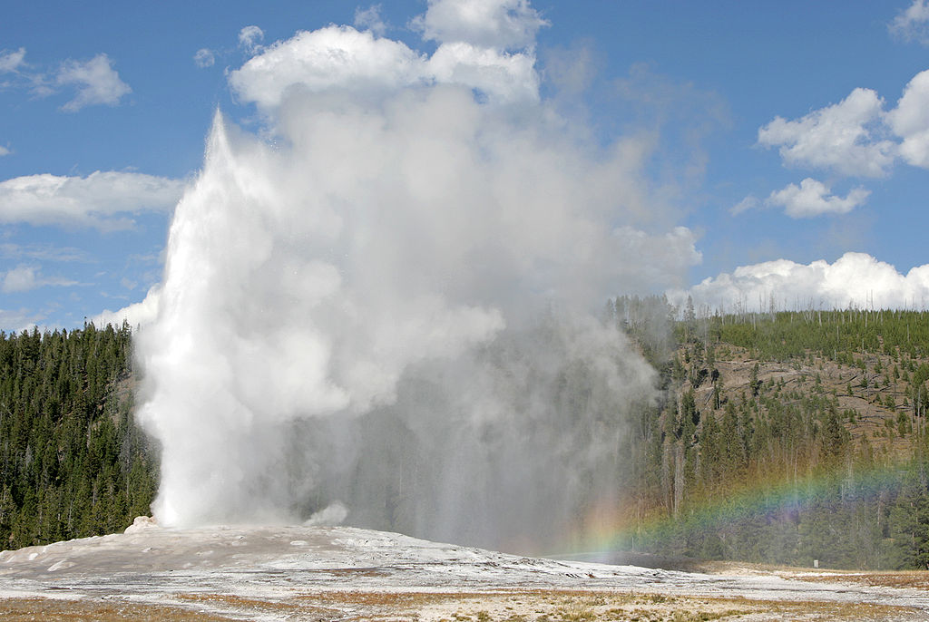
Folks working with time sequence could have heard of Old Faithful, a geyser in
Wyoming, US that has regularly been erupting each 44 minutes to 2 hours for the reason that 12 months 2004. For the subset of knowledge
Gilpin extracted,

geyser_train_test.pkl corresponds to detrended temperature readings from the primary runoff pool of the Previous Devoted geyser
in Yellowstone Nationwide Park, downloaded from the GeyserTimes database. Temperature measurements
begin on April 13, 2015 and happen in one-minute increments.

Like we stated above, geyser.csv is a subset of those measurements, comprising the primary 10000 knowledge factors. To decide on an
enough timestep for the LSTMs, we examine the sequence at varied resolutions:

Determine 1: Geyer dataset. Prime: First 1000 observations. Backside: Zooming in on the primary 200.

It looks as if the habits is periodic with a interval of about 40-50; a timestep of 60 thus appeared like a superb attempt.

Having skilled each FNN-LSTM and the vanilla LSTM for 200 epochs, we first examine the variances of the latent variables on
the check set. The worth of fnn_multiplier similar to this run was 0.7.

test_batch <- as_iterator(ds_test) %>% iter_next()
encoded <- encoder(test_batch[[1]]) %>%
  as.array() %>%
  as_tibble()

encoded %>% summarise_all(var)

   V1     V2        V3          V4       V5       V6       V7       V8       V9      V10
0.258 0.0262 0.0000627 0.000000600 0.000533 0.000362 0.000238 0.000121 0.000518 0.000365

There’s a drop in significance between the primary two variables and the remaining; nevertheless, in contrast to within the Lorenz system, V1 and
V2 variances additionally differ by an order of magnitude.

Now, it’s fascinating to match prediction errors for each fashions. We’re going to make a remark that may carry
via to all three datasets to return.

Maintaining the suspense for some time, right here is the code used to compute per-timestep prediction errors from each fashions. The
similar code will probably be used for all different datasets.

calc_mse <- perform(df, y_true, y_pred) {
  (sum((df[[y_true]] - df[[y_pred]])^2))/nrow(df)
}

get_mse <- perform(test_batch, prediction) {
  
  comp_df <- 
    data.frame(
      test_batch[[2]][, , 1] %>%
        as.array()) %>%
        rename_with(perform(title) paste0(title, "_true")) %>%
    bind_cols(
      data.frame(
        prediction[, , 1] %>%
          as.array()) %>%
          rename_with(perform(title) paste0(title, "_pred")))
  
  mse <- purrr::map(1:dim(prediction)[2],
                        perform(varno)
                          calc_mse(comp_df,
                                   paste0("X", varno, "_true"),
                                   paste0("X", varno, "_pred"))) %>%
    unlist()
  
  mse
}

prediction_fnn <- decoder(encoder(test_batch[[1]]))
mse_fnn <- get_mse(test_batch, prediction_fnn)

prediction_lstm <- mannequin %>% predict(ds_test)
mse_lstm <- get_mse(test_batch, prediction_lstm)

mses <- data.frame(timestep = 1:n_timesteps, fnn = mse_fnn, lstm = mse_lstm) %>%
  collect(key = "sort", worth = "mse", -timestep)

ggplot(mses, aes(timestep, mse, coloration = sort)) +
  geom_point() +
  scale_color_manual(values = c("#00008B", "#3CB371")) +
  theme_classic() +
  theme(legend.place = "none") 

And right here is the precise comparability. One factor particularly jumps to the attention: FNN-LSTM forecast error is considerably decrease for
preliminary timesteps, at the start, for the very first prediction, which from this graph we anticipate to be fairly good!

Determine 2: Per-timestep prediction error as obtained by FNN-LSTM and a vanilla stacked LSTM. Inexperienced: LSTM. Blue: FNN-LSTM.

Curiously, we see “jumps” in prediction error, for FNN-LSTM, between the very first forecast and the second, after which
between the second and the following ones, reminding of the same jumps in variable significance for the latent code! After the
first ten timesteps, vanilla LSTM has caught up with FNN-LSTM, and we gained’t interpret additional growth of the losses based mostly
on only a single run’s output.

As a substitute, let’s examine precise predictions. We randomly decide sequences from the check set, and ask each FNN-LSTM and vanilla
LSTM for a forecast. The identical process will probably be adopted for the opposite datasets.

given <- data.frame(as.array(tf$concat(list(
  test_batch[[1]][, , 1], test_batch[[2]][, , 1]
),
axis = 1L)) %>% t()) %>%
  add_column(sort = "given") %>%
  add_column(num = 1:(2 * n_timesteps))

fnn <- data.frame(as.array(prediction_fnn[, , 1]) %>%
                    t()) %>%
  add_column(sort = "fnn") %>%
  add_column(num = (n_timesteps  + 1):(2 * n_timesteps))

lstm <- data.frame(as.array(prediction_lstm[, , 1]) %>%
                     t()) %>%
  add_column(sort = "lstm") %>%
  add_column(num = (n_timesteps + 1):(2 * n_timesteps))

compare_preds_df <- bind_rows(given, lstm, fnn)

plots <- 
  purrr::map(sample(1:dim(compare_preds_df)[2], 16),
             perform(v) {
               ggplot(compare_preds_df, aes(num, .knowledge[[paste0("X", v)]], coloration = sort)) +
                 geom_line() +
                 theme_classic() +
                 theme(legend.place = "none", axis.title = element_blank()) +
                 scale_color_manual(values = c("#00008B", "#DB7093", "#3CB371"))
             })

plot_grid(plotlist = plots, ncol = 4)

Listed here are sixteen random picks of predictions on the check set. The bottom reality is displayed in pink; blue forecasts are from
FNN-LSTM, inexperienced ones from vanilla LSTM.

Determine 3: 60-step forward predictions from FNN-LSTM (blue) and vanilla LSTM (inexperienced) on randomly chosen sequences from the check set. Pink: the bottom reality.

What we anticipate from the error inspection comes true: FNN-LSTM yields considerably higher predictions for instant
continuations of a given sequence.

Let’s transfer on to the second dataset on our record.

Electrical energy dataset

It is a dataset on energy consumption, aggregated over 321 completely different households and fifteen-minute-intervals.

electricity_train_test.pkl corresponds to common energy consumption by 321 Portuguese households between 2012 and 2014, in
models of kilowatts consumed in fifteen minute increments. This dataset is from the UCI machine learning
database.

Right here, we see a really common sample:

Determine 4: Electrical energy dataset. Prime: First 2000 observations. Backside: Zooming in on 500 observations, skipping the very starting of the sequence.

With such common habits, we instantly tried to foretell a better variety of timesteps (120) – and didn’t should retract
behind that aspiration.

For an fnn_multiplier of 0.5, latent variable variances seem like this:

V1          V2            V3       V4       V5            V6       V7         V8      V9     V10
0.390 0.000637 0.00000000288 1.48e-10 2.10e-11 0.00000000119 6.61e-11 0.00000115 1.11e-4 1.40e-4

We undoubtedly see a pointy drop already after the primary variable.

How do prediction errors examine on the 2 architectures?

Determine 5: Per-timestep prediction error as obtained by FNN-LSTM and a vanilla stacked LSTM. Inexperienced: LSTM. Blue: FNN-LSTM.

Right here, FNN-LSTM performs higher over an extended vary of timesteps, however once more, the distinction is most seen for instant
predictions. Will an inspection of precise predictions verify this view?

Determine 6: 60-step forward predictions from FNN-LSTM (blue) and vanilla LSTM (inexperienced) on randomly chosen sequences from the check set. Pink: the bottom reality.

It does! Actually, forecasts from FNN-LSTM are very spectacular on all time scales.

Now that we’ve seen the simple and predictable, let’s method the bizarre and troublesome.

ECG dataset

Says Gilpin,

ecg_train.pkl and ecg_test.pkl correspond to ECG measurements for 2 completely different sufferers, taken from the PhysioNet QT
database.

How do these look?

Determine 7: ECG dataset. Prime: First 1000 observations. Backside: Zooming in on the primary 400 observations.

To the layperson that I’m, these don’t look practically as common as anticipated. First experiments confirmed that each architectures
aren’t able to coping with a excessive variety of timesteps. In each attempt, FNN-LSTM carried out higher for the very first
timestep.

That is additionally the case for n_timesteps = 12, the ultimate attempt (after 120, 60 and 30). With an fnn_multiplier of 1, the
latent variances obtained amounted to the next:

     V1        V2          V3        V4         V5       V6       V7         V8         V9       V10
  0.110  1.16e-11     3.78e-9 0.0000992    9.63e-9  4.65e-5  1.21e-4    9.91e-9    3.81e-9   2.71e-8

There is a spot between the primary variable and all different ones; however not a lot variance is defined by V1 both.

Other than the very first prediction, vanilla LSTM exhibits decrease forecast errors this time; nevertheless, we’ve got so as to add that this
was not constantly noticed when experimenting with different timestep settings.

Determine 8: Per-timestep prediction error as obtained by FNN-LSTM and a vanilla stacked LSTM. Inexperienced: LSTM. Blue: FNN-LSTM.

Taking a look at precise predictions, each architectures carry out greatest when a persistence forecast is enough – in truth, they
produce one even when it’s not.

Determine 9: 60-step forward predictions from FNN-LSTM (blue) and vanilla LSTM (inexperienced) on randomly chosen sequences from the check set. Pink: the bottom reality.

On this dataset, we definitely would wish to discover different architectures higher in a position to seize the presence of excessive and low
frequencies within the knowledge, reminiscent of combination fashions. However – had been we pressured to stick with one among these, and will do a
one-step-ahead, rolling forecast, we’d go together with FNN-LSTM.

Talking of blended frequencies – we haven’t seen the extremes but …

Mouse dataset

“Mouse,” that’s spike charges recorded from a mouse thalamus.

mouse.pkl A time sequence of spiking charges for a neuron in a mouse thalamus. Uncooked spike knowledge was obtained from
CRCNS and processed with the authors’ code with a purpose to generate a
spike charge time sequence.

Determine 10: Mouse dataset. Prime: First 2000 observations. Backside: Zooming in on the primary 500 observations.

Clearly, this dataset will probably be very exhausting to foretell. How, after “lengthy” silence, are you aware {that a} neuron goes to fireside?

As typical, we examine latent code variances (fnn_multiplier was set to 0.4):

     V1       V2        V3         V4       V5       V6        V7      V8       V9        V10
 0.0796  0.00246  0.000214    2.26e-7   .71e-9  4.22e-8  6.45e-10 1.61e-4 2.63e-10    2.05e-8
>

Again, we don’t see the first variable explaining much variance. Still, interestingly, when inspecting forecast errors we get
a picture very similar to the one obtained on our first, geyser, dataset:

Figure 11: Per-timestep prediction error as obtained by FNN-LSTM and a vanilla stacked LSTM. Green: LSTM. Blue: FNN-LSTM.

So here, the latent code definitely seems to help! With every timestep “more” that we try to predict, prediction performance
goes down continuously – or put the other way round, short-time predictions are expected to be pretty good!

Let’s see:

Figure 12: 60-step ahead predictions from FNN-LSTM (blue) and vanilla LSTM (green) on randomly selected sequences from the test set. Pink: the ground truth.

In fact on this dataset, the difference in behavior between both architectures is striking. When nothing is “supposed to
happen,” vanilla LSTM produces “flat” curves at about the mean of the data, while FNN-LSTM takes the effort to “stay on track”
as long as possible before also converging to the mean. Choosing FNN-LSTM – had we to choose one of these two – would be an
obvious decision with this dataset.

Discussion

When, in timeseries forecasting, would we consider FNN-LSTM? Judging by the above experiments, conducted on four very different
datasets: Whenever we consider a deep learning approach. Of course, this has been a casual exploration – and it was meant to
be, as – hopefully – was evident from the nonchalant and bloomy (sometimes) writing style.

Throughout the text, we’ve emphasized utility – how could this technique be used to improve predictions? But, looking at
the above results, a number of interesting questions come to mind. We already speculated (though in an indirect way) whether
the number of high-variance variables in the latent code was relatable to how far we could sensibly forecast into the future.
However, even more intriguing is the question of how characteristics of the dataset itself affect FNN efficiency.

Such characteristics could be:

• How nonlinear is the dataset? (Put differently, how incompatible, as indicated by some form of test algorithm, is it with
  the hypothesis that the data generation mechanism was a linear one?)

• To what degree does the system appear to be sensitively dependent on initial conditions? In other words, what is the value
  of its (estimated, from the observations) highest Lyapunov exponent?

• What’s its (estimated) dimensionality, for instance, when it comes to correlation
  dimension?

Whereas it’s straightforward to acquire these estimates, utilizing, for example, the
nonlinearTseries package deal explicitly modeled after practices
described in Kantz & Schreiber’s basic (Kantz and Schreiber 2004), we don’t wish to extrapolate from our tiny pattern of datasets, and go away
such explorations and analyses to additional posts, and/or the reader’s ventures :-). In any case, we hope you loved
the demonstration of sensible usability of an method that within the previous publish, was primarily launched when it comes to its
conceptual attractivity.

Thanks for studying!