Time Sequence Knowledge Evaluation with sARIMA and Sprint | by Gabriele Albini | Might, 2023

1.1 The constructing blocks of the mannequin

To grasp what sARIMA fashions are, let’s first introduce the constructing blocks of those fashions.

sARIMA is a composition of various sub-models (i.e. polynomials that we use to characterize our time collection information) which kind the acronym: seasonal (s) autoregressive (AR) built-in (I) shifting common (MA):

• AR: the autoregressive element, ruled by the hyperparameter “p”, assumes that the present worth at a time “t” may be expressed as a linear mixture of the earlier “p” values:

• I: the built-in element is represented by the hyperparameter “d”, which is the diploma of the differencing transformation utilized to the info. Differencing is a way used to take away development from the info (i.e. make the info stationary with respect to the imply, as we’ll see later), which helps the mannequin match the info because it isolates the development element (we use d=1 for linear development, d=2 for quadratic development, …). Differencing the info with d=1 means working with the distinction between consecutive information factors:

• MA: the shifting common element, ruled by the hyperparameter “q”, assumes that the present worth at a time “t” may be expressed as a continuing time period (often the imply) plus a linear mixture of the errors of the earlier “q” factors:

• If we take into account the elements up to now, we get “ARIMA”, which is the title of a mannequin household to work with time collection information with no seasonality. sARIMA fashions are a generalization to work with seasonal information with the addition of an S-component: the seasonal element, which consists of a brand new set of AR, I, MA elements with a seasonal lag. In different phrases, as soon as recognized a seasonality and outlined its lag (represented by the hyperparameter “m” — e.g. m=12 implies that yearly, on a month-to-month dataset, we see the identical habits), we create a brand new set of AR (P), I (D), MA (Q) elements, with respect to the seasonal lag (m) (e.g. if D=1 and m=12, which means that we apply a 1-degree differencing to the collection, with a lag of 12).

To sum up, the sARIMA mannequin is outlined by 7 hyperparameters: 3 for the non-seasonal a part of the mannequin, and 4 for the seasonal half. They’re indicated as:

sARIMA (p,d,q) (P,D,Q)m

Due to the mannequin flexibility, we will “change off” the elements that aren’t embodied in our information (i.e. if the info doesn’t have a development or doesn’t have seasonality, the respective parameters may be set to 0) and nonetheless use the identical mannequin framework to suit the info.

Alternatively, amongst sARIMA limitations, we’ve that these fashions can seize just one seasonality. If a day by day dataset has a yearly plus a weekly seasonality, we’ll want to decide on the strongest one.

1.2 How to decide on the mannequin hyperparameters: ACF and PACF

To determine the mannequin hyperparameters, we usually have a look at the autocorrelation and partial-autocorrelation of the time collection; since all of the above elements use previous information to mannequin current and future factors, we should always examine how previous and current information are correlated and outline what number of previous information factors we’d like, to mannequin the current.

For that reason, autocorrelation and partial-autocorrelation are two broadly used capabilities:

• ACF (autocorrelation): describes the correlation of the time collection, with its lags. All information factors are in comparison with their earlier lag 1, lag 2, lag 3, … The ensuing correlation is plotted on a histogram. This chart (additionally referred to as “correlogram”) is used to visualise how a lot data is retained all through the time collection. The ACF helps us in selecting the sARIMA mannequin as a result of:

The ACF helps to determine the MA(q) hyperparameter.

• PACF (partial autocorrelation): describes the partial correlation of the time collection, with its lags. Otherwise from the ACF, the PACF reveals the correlation between some extent X_t and a lag, which isn’t defined by frequent correlations with different lags at a decrease order. In different phrases, the PACF isolates the direct correlation between two phrases. The PACF helps us in selecting the sARIMA mannequin as a result of:

The PACF helps to determine the AR(p) hyperparameter.

Earlier than utilizing these instruments, nonetheless, we have to point out that ACF and PACF can solely be used on a “stationary” time collection.

1.3 Stationarity

A (weakly) stationary time collection is a time collection the place:

• The imply is fixed over time (i.e. the collection fluctuates round a horizontal line with out optimistic or unfavorable developments)
• The variance is fixed over time (i.e. there is no such thing as a seasonality or change within the deviation from the imply)

After all not all time collection are natively stationary; nonetheless, we will rework them to make them stationary. The commonest transformations used to make a time collection stationary are:

• The pure log: by making use of the log to every information level, we often handle to make the time collection stationary with respect to the variance.
• Differencing: by differencing a time collection, we often handle to take away the development and make the time collection stationary with respect to the imply.

After reworking the time collection, we will use two instruments to substantiate that it’s stationary:

• The Field-Cox plot: this can be a plot of the rolling imply (on the x-axis) vs the rolling normal deviation (on the y-axis) (or the imply vs variance of grouped factors). Our information is stationary if we don’t observe any specific developments within the chart and we see little variation on each axes.
• The Augmented Dickey–Fuller take a look at (ADF): a statistical take a look at through which we attempt to reject the null speculation stating that the time collection is non-stationary.

As soon as a time collection is stationary, we will analyze the ACF and PACF patterns, and discover the SARIMA mannequin hyperparameters.

Figuring out the sARIMA mannequin that matches our information include a collection of steps, which we are going to carry out on the AirPassenger dataset (obtainable here).

Every step roughly corresponds to a “web page” of the Sprint internet app.

2.1 Plot your information

Create a line chart of your uncooked information: a number of the options described above may be seen by the bare eye, particularly stationarity, and seasonality.

Within the above chart, we see a optimistic linear development and a recurrent seasonality sample; contemplating that we’ve month-to-month information, we will assume the seasonality to be yearly (lag 12). The information isn’t stationary.

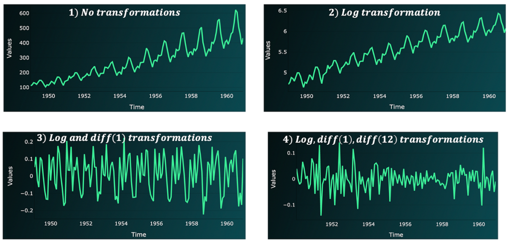
2.2 Rework the info to make it stationary

With a purpose to discover the mannequin hyperparameters, we have to work with a stationary time collection. So, if the info isn’t stationary, we’ll want to rework it:

• Begin with the log transformation, to make the info stationary with respect to the variance (the log is outlined over optimistic values. So, if the info presents unfavorable or 0 values, add a continuing to every datapoint).
• Apply differencing to make the info stationary with respect to the imply. Often begin with differencing of order 1 and lag 1. Then, if information remains to be not stationary, attempt differencing with respect to the seasonal lag (e.g. 12 if we’ve month-to-month information). (Utilizing a reverse order received’t make a distinction).

With our dataset, we have to carry out the next steps to make it totally stationary:

After every step, by wanting on the ADF take a look at p-value and Field-Cox plot, we see that:

• The Field-Cox plot will get progressively cleaned from any development and all factors get nearer and nearer.
• The p-value progressively drops. We are able to lastly reject the null speculation of the take a look at.

2.3 Determine appropriate mannequin hyperparameters with the ACF and PACF

Whereas reworking the info to stationary, we’ve already recognized 3 parameters:

• Since we utilized differencing, the mannequin will embrace differencing elements. We utilized a differencing of 1 and 12: we will set d=1 and D=1 with m=12 (seasonality of 12).

For the remaining parameters, we will have a look at the ACF and PACF after the transformations.

Generally, we will apply the next guidelines:

• We now have an AR(p) course of if: the PACF has a major spike at a sure lag “p” (and no important spikes after) and the ACF decays or reveals a sinusoidal habits (alternating optimistic, unfavorable spikes).
• We now have a MA(q) course of if: the ACF has a major spike at a sure lag “q” (and no important spikes after) and the PACF decays or reveals a sinusoidal habits (alternating optimistic, unfavorable spikes).
• Within the case of seasonal AR(P) or MA(Q) processes, we are going to see that the numerous spikes repeat on the seasonal lags.

By our instance, we see the next:

• The closest rule to the above habits, suggests some MA(q) course of with “q” between 1 and three; the truth that we nonetheless have a major spike at 12, can also counsel an MA(Q) with Q=1 (since m=12).

We use the ACF and PACF to get a spread of hyperparameter values that may kind mannequin candidates. We are able to evaluate these completely different mannequin candidates in opposition to our information, and decide the top-performing one.

Within the instance, our mannequin candidates appear to be:

• SARIMA (p,d,q) (P,D,Q)m = (0, 1, 1) (0, 1, 1) 12
• SARIMA (p,d,q) (P,D,Q)m = (0, 1, 3) (0, 1, 1) 12

2.4 Carry out a mannequin grid search to determine optimum hyperparameters

Grid search can be utilized to match a number of mannequin candidates in opposition to one another: we match every mannequin to the info and decide the top-performing one.

To arrange a grid search we have to:

• create an inventory with all doable combos of mannequin hyperparameters, given a spread of values for every hyperparameter.
• match every mannequin and measure its efficiency utilizing a KPI of selection.
• choose the hyperparameters wanting on the top-performing fashions.

In our case, we are going to evaluate mannequin performances utilizing the AIC (Akaike data criterion) rating. This KPI formulation consists of a trade-off between the becoming error (accuracy) and mannequin complexity. Generally, when the complexity is simply too low, the error is excessive, as a result of we over-simplify the mannequin becoming activity; quite the opposite, when complexity is simply too excessive, the error remains to be excessive because of overfitting. A trade-off between these two will enable us to determine the “top-performing” mannequin.

Sensible word: with becoming a sARIMA mannequin, we might want to use the unique dataset with the log transformation (if we’ve utilized it), however we don’t need to use the info with differencing transformations.

We are able to select to order a part of the time collection (often the latest 20% observations) as a take a look at set.

In our instance, primarily based on the beneath hyperparameter ranges, one of the best mannequin is:

SARIMA (p,d,q) (P,D,Q)m = (0, 1, 1) (0, 1, 1) 12

2.5 Ultimate mannequin: match and predictions

We are able to lastly predict information for practice, take a look at, and any future out-of-sample statement. The ultimate plot is:

To verify that we captured all correlations, we will plot the mannequin residuals ACF and PACF:

On this case, some sign from the sturdy seasonality element remains to be current, however many of the remaining lags have a 0 correlation.

The steps described above ought to work on any dataset which might be modeled by means of sARIMA. To recap :

1-Plot & discover your information

2-Apply transformations to make the info stationary (give attention to the left-end charts and the ADF take a look at)

3-Determine appropriate hyperparameters by wanting on the ACF and PACF (right-end charts)

4-Carry out a grid search to pick optimum hyperparameters

5-Match and predict utilizing one of the best mannequin

Obtain the app domestically, add your individual datasets (by changing the .csv file within the information folder) and attempt to match one of the best mannequin.

Thanks for studying!