Multi-label NLP: An Evaluation of Class Imbalance and Loss Perform Approaches
Multi-label NLP refers back to the job of assigning a number of labels to a given textual content enter, fairly than only one label. In conventional NLP duties, comparable to textual content classification or sentiment evaluation, every enter is often assigned a single label primarily based on its content material. Nonetheless, in lots of real-world situations, a chunk of textual content can belong to a number of classes or categorical a number of sentiments concurrently.
Multi-label NLP is essential as a result of it permits us to seize extra nuanced and complicated info from textual content knowledge. For instance, within the area of buyer suggestions evaluation, a buyer evaluation could categorical each optimistic and damaging sentiments on the similar time, or it could contact upon a number of features of a services or products. By assigning a number of labels to such inputs, we are able to achieve a extra complete understanding of the client’s suggestions and take extra focused actions to handle their issues.
This text delves right into a noteworthy case of Provectus’ use of multi-label NLP.
Context:
A shopper approached us with a request to assist them automate labeling documents of a certain type. At first look, the duty seemed to be simple and simply solved. Nonetheless, as we labored on the case, we encountered a dataset with inconsistent annotations. Although our buyer had confronted challenges with various class numbers and modifications of their evaluation group over time, they’d invested important efforts into creating a various dataset with a variety of annotations. Whereas there existed some imbalances and uncertainties within the labels, this dataset supplied a helpful alternative for evaluation and additional exploration.
Let’s take a more in-depth have a look at the dataset, discover the metrics and our strategy, and recap how Provectus solved the issue of multi-label textual content classification.
The dataset has 14,354 observations, with 124 distinctive lessons (labels). Our job is to assign one or a number of lessons to each remark.
Desk 1 gives descriptive statistics for the dataset.
On common, we’ve got about two lessons per remark, with a median of 261 totally different texts describing a single class.
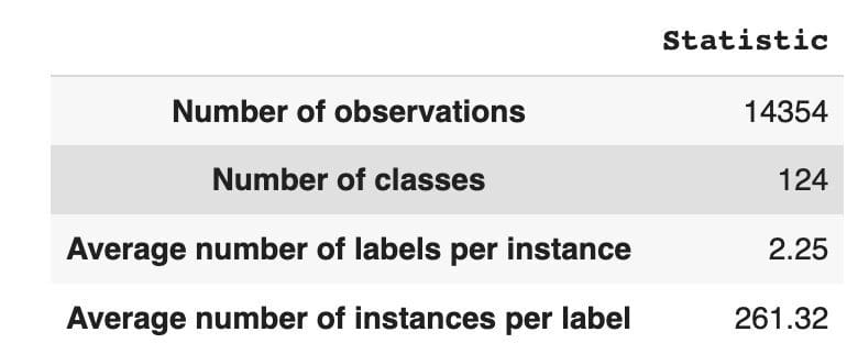
Desk 1: Dataset Statistic
In Determine 1, we see the distribution of lessons within the high graph, and we’ve got a sure variety of HEAD labels with the best frequency of incidence within the dataset. Additionally be aware that almost all of lessons have a low frequency of incidence.
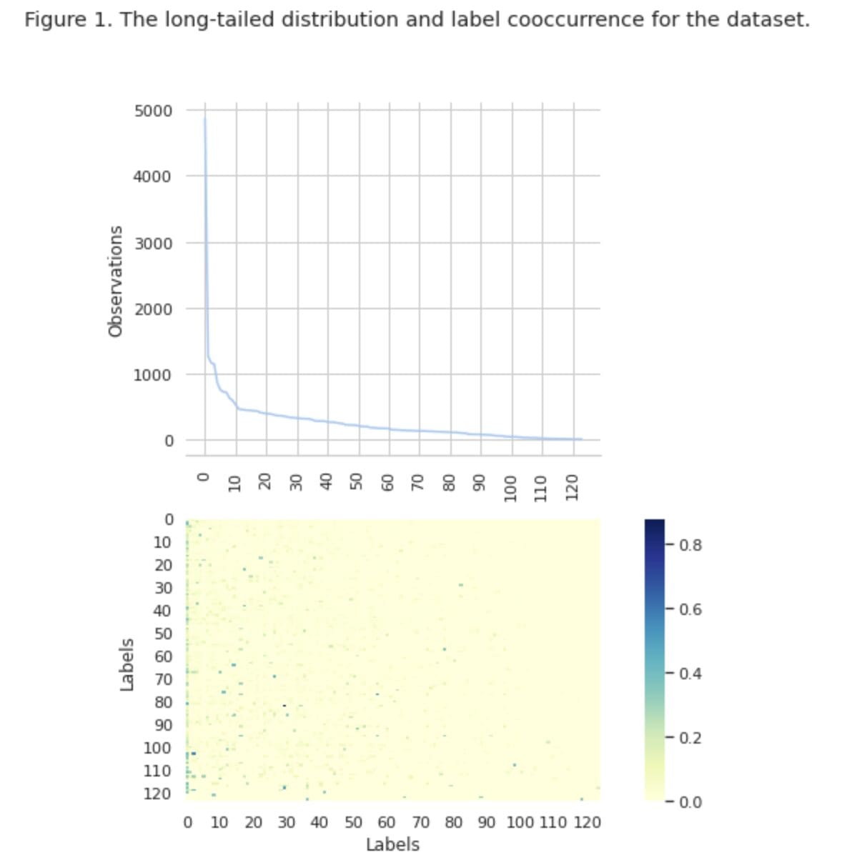
Within the backside graph we see that there’s frequent overlap between the lessons which are finest represented within the dataset, and the lessons which have low significance.
We modified the method of splitting the dataset into prepare/val/check units. As a substitute of utilizing a standard methodology, we’ve got employed iterative stratification, to supply a well-balanced distribution of proof of label relations. For that, we used Scikit Multi-learn
from skmultilearn.model_selection import iterative_train_test_split

mlb = MultiLabelBinarizer()


def balanced_split(df, mlb, test_size=0.5):
    ind = np.expand_dims(np.arange(len(df)), axis=1)
    mlb.fit_transform(df["tag"])
    labels = mlb.remodel(df["tag"])
    ind_train, _, ind_test, _ = iterative_train_test_split(
        ind, labels, test_size
    )
    return df.iloc[ind_train[:, 0]], df.iloc[ind_test[:, 0]]


df_train, df_tmp = balanced_split(df, test_size=0.4)
df_val, df_test = balanced_split(df_tmp, test_size=0.5)
We obtained the next distribution:
- The coaching dataset comprises 60% of the information and covers all 124 labels
- The validation dataset comprises 20% of the information and covers all 124 labels
- The check dataset comprises 20% of the information and covers all 124 labels
Multi-label classification is a kind of supervised machine studying algorithm that permits us to assign a number of labels to a single knowledge pattern. It differs from binary classification the place the mannequin predicts solely two classes, and multi-class classification the place the mannequin predicts just one out of a number of lessons for a pattern.
Analysis metrics for multi-label classification efficiency are inherently totally different from these utilized in multi-class (or binary) classification because of the inherent variations of the classification drawback. Extra detailed info will be discovered on Wikipedia.
We chosen metrics which are best suited for us:
- Precision measures the proportion of true optimistic predictions among the many complete optimistic predictions made by the mannequin.
- Recall measures the proportion of true optimistic predictions amongst all precise optimistic samples.
- F1-score is the harmonic imply of precision and recall, which helps to revive steadiness between the 2.
- Hamming loss is the fraction of labels which are incorrectly predicted
We additionally monitor the variety of predicted labels within the set { outlined as depend for labels, for which we obtain an F1 rating > 0}.
Multi-Label Classification is a kind of supervised studying drawback the place a single occasion or instance will be related to a number of labels or classifications, versus conventional single-label classification, the place every occasion is simply related to a single class label.
To resolve multi-label classification issues, there are two fundamental classes of methods:
- Drawback transformation strategies
- Algorithm adaptation strategies
Drawback transformation strategies allow us to remodel multi-label classification duties into a number of single-label classification duties. For instance, the Binary Relevance (BR) baseline strategy treats each label as a separate binary classification drawback. On this case, the multi-label drawback is reworked into a number of single-label issues.
Algorithm adaptation strategies modify the algorithms themselves to deal with multi-label knowledge natively, with out reworking the duty into a number of single-label classification duties. An instance of this strategy is the BERT model, which is a pre-trained transformer-based language mannequin that may be fine-tuned for numerous NLP duties, together with multi-label textual content classification. BERT is designed to deal with multi-label knowledge straight, with out the necessity for drawback transformation.
Within the context of utilizing BERT for multi-label textual content classification, the usual strategy is to make use of Binary Cross-Entropy (BCE) loss because the loss operate. BCE loss is a generally used loss operate for binary classification issues and will be simply prolonged to deal with multi-label classification issues by computing the loss for every label independently, after which summing the losses. On this case, the BCE loss operate measures the error between predicted chances and true labels, the place predicted chances are obtained from the ultimate sigmoid activation layer within the BERT mannequin.
Now, let’s take a more in-depth have a look at Determine 2 under.
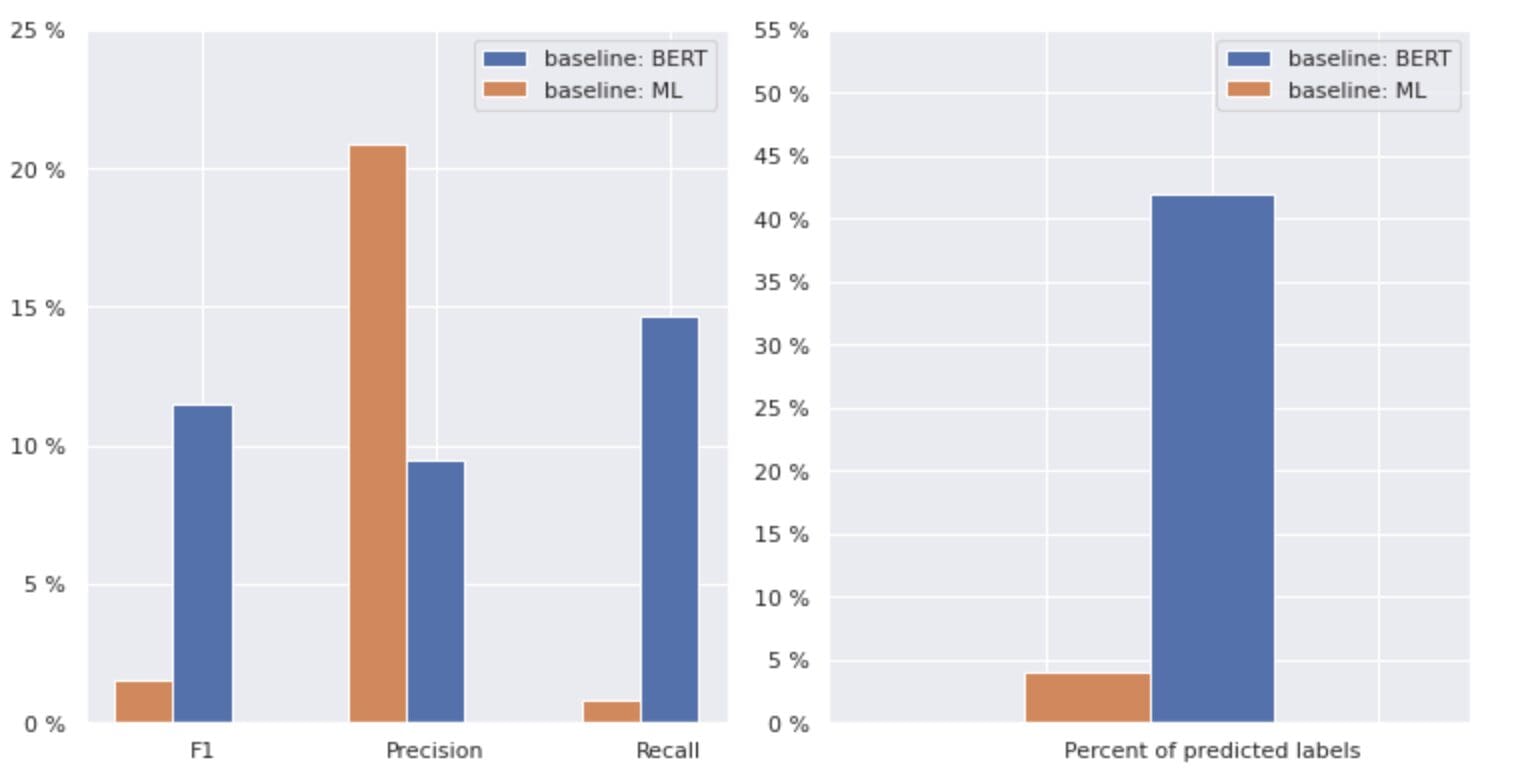
Determine 2. Metrics for baseline fashions
The graph on the left exhibits a comparability of metrics for a “baseline: BERT” and “baseline: ML”. Thus, it may be seen that for “baseline: BERT”, the F1 and Recall scores are roughly 1.5 instances larger, whereas the Precision for “baseline: ML” is 2 instances larger than that of mannequin 1. By analyzing the general proportion of predicted lessons proven on the suitable, we see that “baseline: BERT” predicted lessons greater than 10 instances that of “baseline: ML”.
As a result of the utmost end result for the “baseline: BERT” is lower than 50% of all lessons, the outcomes are fairly discouraging. Let’s work out how you can enhance these outcomes.
Based mostly on the excellent article “Balancing Methods for Multi-label Text Classification with Long-Tailed Class Distribution”, we realized that distribution-balanced loss could be the best suited strategy for us.
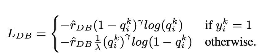
Distribution-balanced loss
Distribution-balanced loss is a way utilized in multi-label textual content classification issues to handle imbalances at school distribution. In these issues, some lessons have a a lot larger frequency of incidence in comparison with others, leading to mannequin bias towards these extra frequent lessons.
To handle this subject, distribution-balanced loss goals to steadiness the contribution of every pattern within the loss operate. That is achieved by re-weighting the lack of every pattern primarily based on the inverse of its frequency of incidence within the dataset. By doing so, the contribution of much less frequent lessons is elevated, and the contribution of extra frequent lessons is decreased, thus balancing the general class distribution.
This system has been proven to be efficient in enhancing the efficiency of fashions on long-tailed class distribution issues. By lowering the affect of frequent lessons and growing the affect of rare lessons, the mannequin is ready to higher seize patterns within the knowledge and produce extra balanced predictions.
Implementation of Resample Class
import torch
import torch.nn as nn
import torch.nn.useful as F
import numpy as np


class ResampleLoss(nn.Module):
    def __init__(
        self,
        use_sigmoid=True,
        partial=False,
        loss_weight=1.0,
        discount="imply",
        reweight_func=None,
        weight_norm=None,
        focal=dict(focal=True, alpha=0.5, gamma=2),
        map_param=dict(alpha=10.0, beta=0.2, gamma=0.1),
        CB_loss=dict(CB_beta=0.9, CB_mode="average_w"),
        logit_reg=dict(neg_scale=5.0, init_bias=0.1),
        class_freq=None,
        train_num=None,
    ):
        tremendous(ResampleLoss, self).__init__()
        assert (use_sigmoid is True) or (partial is False)
        self.use_sigmoid = use_sigmoid
        self.partial = partial
        self.loss_weight = loss_weight
        self.discount = discount
        if self.use_sigmoid:
            if self.partial:
                self.cls_criterion = partial_cross_entropy
            else:
                self.cls_criterion = binary_cross_entropy
        else:
            self.cls_criterion = cross_entropy
        # reweighting operate
        self.reweight_func = reweight_func
        # normalization (optionally available)
        self.weight_norm = weight_norm
        # focal loss params
        self.focal = focal["focal"]
        self.gamma = focal["gamma"]
        self.alpha = focal["alpha"]
        # mapping operate params
        self.map_alpha = map_param["alpha"]
        self.map_beta = map_param["beta"]
        self.map_gamma = map_param["gamma"]
        # CB loss params (optionally available)
        self.CB_beta = CB_loss["CB_beta"]
        self.CB_mode = CB_loss["CB_mode"]
        self.class_freq = (
            torch.from_numpy(np.asarray(class_freq)).float().cuda()
        )
        self.num_classes = self.class_freq.form[0]
        self.train_num = train_num  # solely was once divided by class_freq
        # regularization params
        self.logit_reg = logit_reg
        self.neg_scale = (
            logit_reg["neg_scale"] if "neg_scale" in logit_reg else 1.0
        )
        init_bias = (
            logit_reg["init_bias"] if "init_bias" in logit_reg else 0.0
        )
        self.init_bias = (
            -torch.log(self.train_num / self.class_freq - 1) * init_bias
        )
        self.freq_inv = (
            torch.ones(self.class_freq.form).cuda() / self.class_freq
        )
        self.propotion_inv = self.train_num / self.class_freq

    def ahead(
        self,
        cls_score,
        label,
        weight=None,
        avg_factor=None,
        reduction_override=None,
        **kwargs
    ):
        assert reduction_override in (None, "none", "imply", "sum")
        discount = (
            reduction_override if reduction_override else self.discount
        )
        weight = self.reweight_functions(label)
        cls_score, weight = self.logit_reg_functions(
            label.float(), cls_score, weight
        )
        if self.focal:
            logpt = self.cls_criterion(
                cls_score.clone(),
                label,
                weight=None,
                discount="none",
                avg_factor=avg_factor,
            )
            # pt is sigmoid(logit) for pos or sigmoid(-logit) for neg
            pt = torch.exp(-logpt)
            wtloss = self.cls_criterion(
                cls_score, label.float(), weight=weight, discount="none"
            )
            alpha_t = torch.the place(label == 1, self.alpha, 1 - self.alpha)
            loss = alpha_t * ((1 - pt) ** self.gamma) * wtloss
            loss = reduce_loss(loss, discount)
        else:
            loss = self.cls_criterion(
                cls_score, label.float(), weight, discount=discount
            )
        loss = self.loss_weight * loss
        return loss

    def reweight_functions(self, label):
        if self.reweight_func is None:
            return None
        elif self.reweight_func in ["inv", "sqrt_inv"]:
            weight = self.RW_weight(label.float())
        elif self.reweight_func in "rebalance":
            weight = self.rebalance_weight(label.float())
        elif self.reweight_func in "CB":
            weight = self.CB_weight(label.float())
        else:
            return None
        if self.weight_norm isn't None:
            if "by_instance" in self.weight_norm:
                max_by_instance, _ = torch.max(weight, dim=-1, keepdim=True)
                weight = weight / max_by_instance
            elif "by_batch" in self.weight_norm:
                weight = weight / torch.max(weight)
        return weight

    def logit_reg_functions(self, labels, logits, weight=None):
        if not self.logit_reg:
            return logits, weight
        if "init_bias" in self.logit_reg:
            logits += self.init_bias
        if "neg_scale" in self.logit_reg:
            logits = logits * (1 - labels) * self.neg_scale + logits * labels
            if weight isn't None:
                weight = (
                    weight / self.neg_scale * (1 - labels) + weight * labels
                )
        return logits, weight

    def rebalance_weight(self, gt_labels):
        repeat_rate = torch.sum(
            gt_labels.float() * self.freq_inv, dim=1, keepdim=True
        )
        pos_weight = (
            self.freq_inv.clone().detach().unsqueeze(0) / repeat_rate
        )
        # pos and neg are equally handled
        weight = (
            torch.sigmoid(self.map_beta * (pos_weight - self.map_gamma))
            + self.map_alpha
        )
        return weight

    def CB_weight(self, gt_labels):
        if "by_class" in self.CB_mode:
            weight = (
                torch.tensor((1 - self.CB_beta)).cuda()
                / (1 - torch.pow(self.CB_beta, self.class_freq)).cuda()
            )
        elif "average_n" in self.CB_mode:
            avg_n = torch.sum(
                gt_labels * self.class_freq, dim=1, keepdim=True
            ) / torch.sum(gt_labels, dim=1, keepdim=True)
            weight = (
                torch.tensor((1 - self.CB_beta)).cuda()
                / (1 - torch.pow(self.CB_beta, avg_n)).cuda()
            )
        elif "average_w" in self.CB_mode:
            weight_ = (
                torch.tensor((1 - self.CB_beta)).cuda()
                / (1 - torch.pow(self.CB_beta, self.class_freq)).cuda()
            )
            weight = torch.sum(
                gt_labels * weight_, dim=1, keepdim=True
            ) / torch.sum(gt_labels, dim=1, keepdim=True)
        elif "min_n" in self.CB_mode:
            min_n, _ = torch.min(
                gt_labels * self.class_freq + (1 - gt_labels) * 100000,
                dim=1,
                keepdim=True,
            )
            weight = (
                torch.tensor((1 - self.CB_beta)).cuda()
                / (1 - torch.pow(self.CB_beta, min_n)).cuda()
            )
        else:
            increase NameError
        return weight

    def RW_weight(self, gt_labels, by_class=True):
        if "sqrt" in self.reweight_func:
            weight = torch.sqrt(self.propotion_inv)
        else:
            weight = self.propotion_inv
        if not by_class:
            sum_ = torch.sum(weight * gt_labels, dim=1, keepdim=True)
            weight = sum_ / torch.sum(gt_labels, dim=1, keepdim=True)
        return weight


def reduce_loss(loss, discount):
    """Cut back loss as specified.
    Args:
        loss (Tensor): Elementwise loss tensor.
        discount (str): Choices are "none", "imply" and "sum".
    Return:
        Tensor: Lowered loss tensor.
    """
    reduction_enum = F._Reduction.get_enum(discount)
    # none: 0, elementwise_mean:1, sum: 2
    if reduction_enum == 0:
        return loss
    elif reduction_enum == 1:
        return loss.imply()
    elif reduction_enum == 2:
        return loss.sum()


def weight_reduce_loss(loss, weight=None, discount="imply", avg_factor=None):
    """Apply element-wise weight and scale back loss.
    Args:
        loss (Tensor): Aspect-wise loss.
        weight (Tensor): Aspect-wise weights.
        discount (str): Identical as built-in losses of PyTorch.
        avg_factor (float): Avarage issue when computing the imply of losses.
    Returns:
        Tensor: Processed loss values.
    """
    # if weight is specified, apply element-wise weight
    if weight isn't None:
        loss = loss * weight
    # if avg_factor isn't specified, simply scale back the loss
    if avg_factor is None:
        loss = reduce_loss(loss, discount)
    else:
        # if discount is imply, then common the loss by avg_factor
        if discount == "imply":
            loss = loss.sum() / avg_factor
        # if discount is 'none', then do nothing, in any other case increase an error
        elif discount != "none":
            increase ValueError(
                'avg_factor cannot be used with discount="sum"'
            )
    return loss


def binary_cross_entropy(
    pred, label, weight=None, discount="imply", avg_factor=None
):
    # weighted element-wise losses
    if weight isn't None:
        weight = weight.float()
    loss = F.binary_cross_entropy_with_logits(
        pred, label.float(), weight, discount="none"
    )
    loss = weight_reduce_loss(
        loss, discount=discount, avg_factor=avg_factor
    )

    return loss
loss_func = ResampleLoss(
    reweight_func="rebalance",
    loss_weight=1.0,
    focal=dict(focal=True, alpha=0.5, gamma=2),
    logit_reg=dict(init_bias=0.05, neg_scale=2.0),
    map_param=dict(alpha=0.1, beta=10.0, gamma=0.405),
    class_freq=class_freq,
    train_num=train_num,
)
"""
class_freq - checklist of frequencies for every class,
train_num - measurement of prepare dataset
"""
By carefully investigating the dataset, we’ve got concluded that the parameter
= 0.405.
Threshold tuning
One other step in enhancing our mannequin was the method of tuning the edge, each within the coaching stage, and within the validation and testing levels. We calculated the dependencies of metrics comparable to f1-score, precision, and recall on the edge stage, and we chosen the edge primarily based on the best metric rating. Under you may see the operate implementation of this course of.
Optimization of the F1 rating by tuning the edge:
def optimise_f1_score(true_labels: np.ndarray, pred_labels: np.ndarray):
    best_med_th = 0.5
    true_bools = [tl == 1 for tl in true_labels]
    micro_thresholds = (np.array(vary(-45, 15)) / 100) + best_med_th
    f1_results, pre_results, recall_results = [], [], []
    for th in micro_thresholds:
        pred_bools = [pl > th for pl in pred_labels]
        test_f1 = f1_score(true_bools, pred_bools, common="micro", zero_division=0)
        test_precision = precision_score(
            true_bools, pred_bools, common="micro", zero_division=0
        )
        test_recall = recall_score(
            true_bools, pred_bools, common="micro", zero_division=0
        )
        f1_results.append(test_f1)
        prec_results.append(test_precision)
        recall_results.append(test_recall)
        best_f1_idx = np.argmax(f1_results)
    return micro_thresholds[best_f1_idx]
Analysis and comparability with baseline
These approaches allowed us to coach a brand new mannequin and procure the next end result, which is in comparison with the baseline: BERT in Determine 3 under.
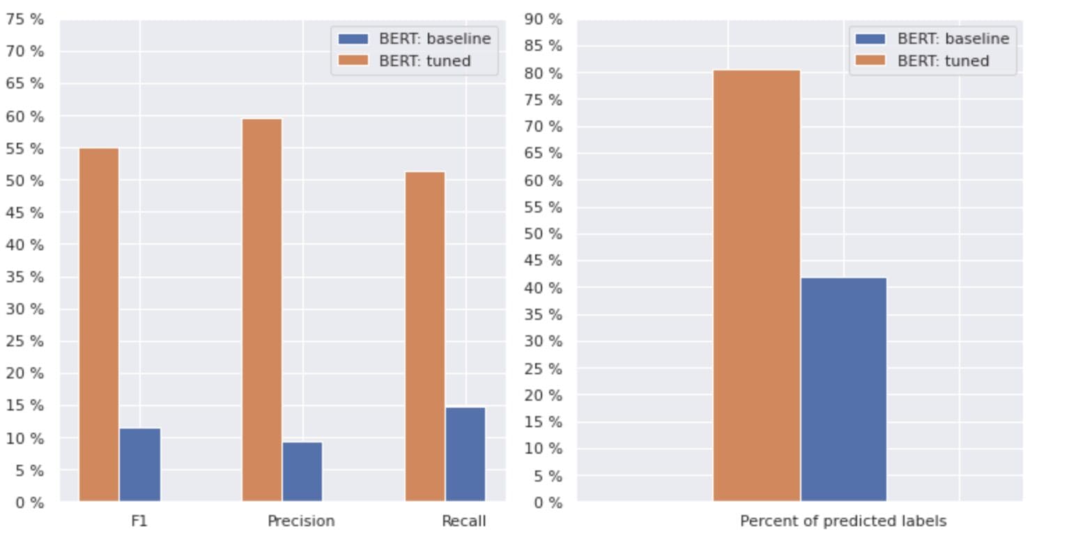
Determine 3. Comparability metrics by baseline and newer strategy.
By evaluating the metrics which are related for classification, we see a major enhance in efficiency measures nearly by 5-6 instances:
The F1 rating elevated from 12% → 55%, whereas Precision elevated from 9% → 59% and Recall elevated from 15% → 51%.
With the modifications proven in the suitable graph in Determine 3, we are able to now predict 80% of the lessons.
Slices of lessons
We divided our labels into 4 teams: HEAD, MEDIUM, TAIL, and ZERO. Every group comprises labels with the same quantity of supporting knowledge observations.
As seen in Determine 4, the distributions of the teams are distinct. The rose field (HEAD) has a negatively skewed distribution, the middlebox (MEDIUM) has a positively skewed distribution, and the inexperienced field (TAIL) seems to have a traditional distribution.
All teams even have outliers, that are factors exterior the whiskers within the field plot. The HEAD group has a serious affect on a MAJOR class.
Moreover, we’ve got recognized a separate group named “ZERO” which comprises labels that the mannequin was unable to study and can’t acknowledge because of the minimal variety of occurrences within the dataset (lower than 3% of all observations).
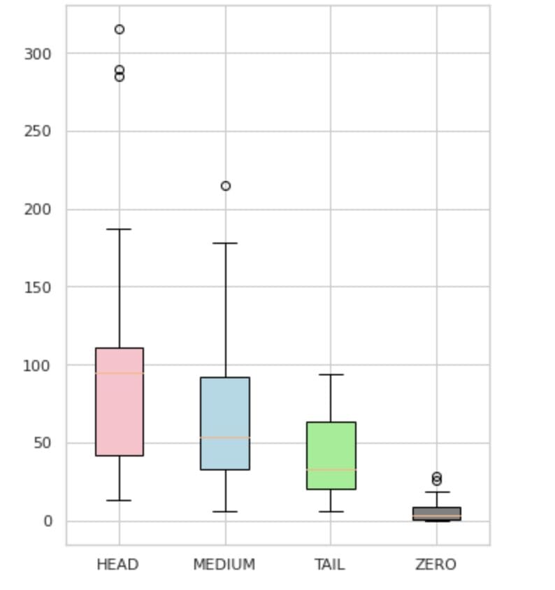
Determine 4. Label counts vs. teams
Desk 2 gives details about metrics per every group of labels for the check subset of information.

Desk 2. Metrics per group.
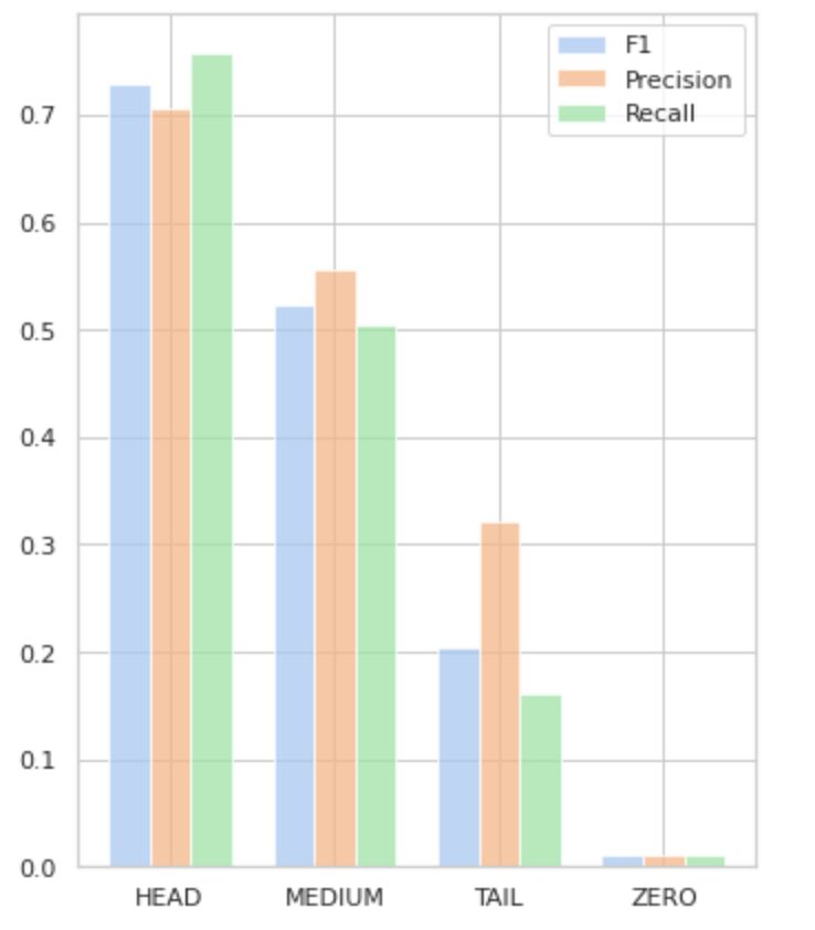
- The HEAD group comprises 21 labels with a median of 112 assist observations per label. This group is impacted by outliers and, on account of its excessive illustration within the dataset, its metrics are excessive: F1 – 73%, Precision – 71%, Recall – 75%.
- The MEDIUM group consists of 44 labels with a median assist of 67 observations, which is roughly two instances decrease than the HEAD group. The metrics for this group are anticipated to lower by 50%: F1 – 52%, Precision – 56%, Recall – 51%.
- The TAIL group has the most important variety of lessons, however all are poorly represented within the dataset, with a median of 40 assist observations per label. In consequence, the metrics drop considerably: F1 – 21%, Precision – 32%, Recall – 16%.
- The ZERO group contains lessons that the mannequin can’t acknowledge in any respect, doubtlessly on account of their low incidence within the dataset. Every of the 24 labels on this group has a median of seven assist observations.
Determine 5 visualizes the data offered in Desk 2, offering a visible illustration of the metrics per group of labels.

Determine 5. Metrics vs. label teams. All ZERO values = 0.
On this complete article, we’ve got demonstrated {that a} seemingly easy job of multi-label textual content classification will be difficult when conventional strategies are utilized. We now have proposed the usage of distribution-balancing loss features to deal with the difficulty of sophistication imbalance.
We now have in contrast the efficiency of our proposed strategy to the basic methodology, and evaluated it utilizing real-world enterprise metrics. The outcomes reveal that using loss features to handle class imbalances and label co-occurrences provide a viable resolution for multi-label textual content classification.
The proposed use case highlights the significance of contemplating totally different approaches and methods when coping with multi-label textual content classification, and the potential advantages of distribution-balancing loss features in addressing class imbalances.
In case you are going through the same subject and searching for to streamline document processing operations inside your group, please contact me or the Provectus group. We might be comfortable to help you to find extra environment friendly strategies for automating your processes.
Oleksii Babych is a Machine Studying Engineer at Provectus. With a background in physics, he possesses wonderful analytical and math abilities, and has gained helpful expertise by scientific analysis and worldwide convention shows, together with SPIE Photonics West. Oleksii focuses on creating end-to-end, large-scale AI/ML options for healthcare and fintech industries. He’s concerned in each stage of the ML growth life cycle, from figuring out enterprise issues to deploying and operating manufacturing ML fashions.
Rinat Akhmetov is the ML Answer Architect at Provectus. With a strong sensible background in Machine Studying (particularly in Laptop Imaginative and prescient), Rinat is a nerd, knowledge fanatic, software program engineer, and workaholic whose second largest ardour is programming. At Provectus, Rinat is in command of the invention and proof of idea phases, and leads the execution of advanced AI initiatives.