The way to Regularize Your Regression – Machine Studying Weblog | ML@CMU
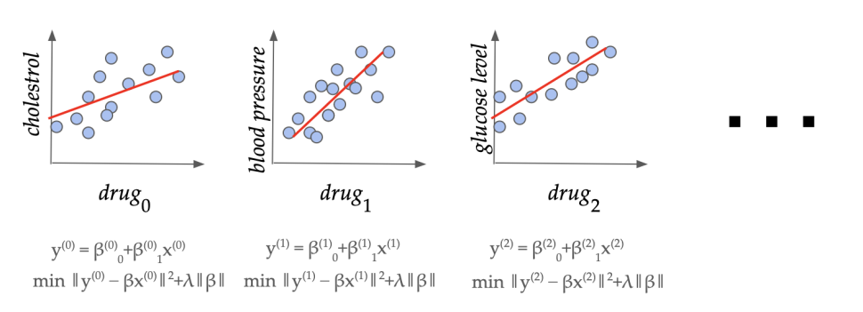
A sequence of regression cases in a pharmaceutical software. Can we learn to set the regularization parameter (lambda) from related domain-specific information?
Overview. Maybe the only relation between an actual dependent variable (y) and a vector of options (X) is a linear mannequin (y = beta X). Given some coaching examples or datapoints consisting of pairs of options and dependent variables ((X_1, y_1),(X_2, y_2),dots,(X_m,y_m)), we want to be taught (beta) which might give the very best prediction (y’) given options (X’) of an unseen instance. This technique of becoming a linear mannequin (beta) to the datapoints is known as linear regression. This straightforward but efficient mannequin finds ubiquitous functions, starting from organic, behavioral, and social sciences to environmental research and monetary forecasting, to make dependable predictions on future information. In ML terminology, linear regression is a supervised studying algorithm with low variance and good generalization properties. It’s a lot much less data-hungry than typical deep studying fashions, and performs properly even with small quantities of coaching information. Additional, to keep away from overfitting the mannequin to the coaching information, which reduces the prediction efficiency on unseen information, one sometimes makes use of regularization, which modifies the target perform of the linear mannequin to scale back affect of outliers and irrelevant options (learn on for particulars).
The most typical methodology for linear regression is “regularized least squares”, the place one finds the (beta) which minimizes
$$||y – beta X||_2^2 + lambda ||beta||.$$
Right here the primary time period captures the error of (beta) on the coaching set, and the second time period is a norm-based penalty to keep away from overfitting (e.g. decreasing affect of outliers in information). The way to set (lambda) appropriately on this elementary methodology relies on the information area and is a longstanding open question. In typical fashionable functions, we’ve got entry to a number of related datasets (X^{(0)},y^{(0)}, X^{(1)},y^{(1)}, dots) from the identical software area. For instance, there are sometimes a number of drug trial research in a pharmaceutical firm for finding out the totally different results of comparable medication. On this work, we present that we will certainly be taught an excellent domain-specific worth of (lambda) with sturdy theoretical ensures of accuracy on unseen datasets from the identical area, and provides bounds on how a lot information is required to attain this.
As our principal outcome, we present that if the information has (p) options (i.e., the dimension of function vector (X_i) is (p), then after seeing (O(p/epsilon^2)) datasets, we will be taught a price of (lambda) which has error (averaged over the area) inside (epsilon) of the very best worth of (lambda) for the area. We additionally lengthen our outcomes to sequential information, binary classification (i.e. (y) is binary valued) and non-linear regression.
Drawback Setup. Linear regression with norm-based regularization penalty is among the hottest methods that one encounters in introductory programs to statistics or machine studying. It’s extensively used for information evaluation and have choice, with quite a few functions together with medicine, quantitative finance (the linear factor model), climate science, and so forth. The regularization penalty is often a weighted additive time period (or phrases) of the norms of the realized linear mannequin (beta), the place the load is rigorously chosen by a site professional. Mathematically, a dataset has dependent variable (y) consisting of (m) examples, and predictor variables (X) with (p) options for every of the (m) datapoints. The linear regression method (with squared loss) consists of fixing a minimization downside
$$hat{beta}^{X,y}_{lambda_1,lambda_2}=textual content{argmin}_{betainmathbb{R}^p}||y-Xbeta||^2+lambda_1||beta||_1+lambda_2||beta||_2^2,$$
the place the highlighted time period is the regularization penalty. Right here (lambda_1, lambda_2ge 0) are the regularization coefficients constraining the L1 and L2 norms, respectively, of the realized linear mannequin (beta). For basic (lambda_1) and (lambda_2) the above algorithm is popularly generally known as the Elastic Net, whereas setting (lambda_1 = 0) recovers Ridge regression and setting (lambda_2 = 0) corresponds to LASSO. Ridge and LASSO regression are each individually well-liked strategies in observe, and the Elastic Web incorporates the benefits of each.
Regardless of the central position these coefficients play in linear regression, the issue of setting them in a principled manner has been a difficult open downside for a number of a long time. In observe, one sometimes makes use of “grid search” cross-validation, which includes (1) splitting the dataset into a number of subsets consisting of coaching and validation units, (2) coaching a number of fashions (comparable to totally different values of regularization coefficients) on every coaching set, and (3) evaluating the efficiency of the fashions on the corresponding validation units. This method has a number of limitations.
- First, that is very computationally intensive, particularly with the massive datasets that typical fashionable functions contain, as one wants to coach and consider the mannequin for a lot of hyperparameter values and training-validation splits. We want to keep away from repeating this cumbersome course of for related functions.
- Second, theoretical ensures on how properly the coefficients realized by this process will carry out on unseen examples should not recognized, even when the check information are drawn from the identical distribution because the coaching set.
- Lastly, this may solely be achieved for a finite set of hyperparameter values and it isn’t clear how the chosen parameter compares to the very best parameter from the continual area of coefficients. Particularly, the loss as a perform of the regularization parameter just isn’t recognized to be Lipschitz.
Our work addresses all three of the above limitations concurrently within the data-driven setting, which we encourage and describe subsequent.
The significance of regularization
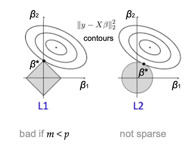
A visualization of the L1 and L2 regularized regressions.
The regularization coefficients (lambda_1) and (lambda_2) play a vital position throughout fields: In machine learning, controlling the norm of mannequin weights (beta) implies provable generalization ensures and prevents over-fitting in observe. In statistical data analysis, their mixed use yields parsimonious and interpretable fashions. In Bayesian statistics they correspond to imposing particular priors on (beta). Successfully, (lambda_2) regularizes (beta) by uniformly shrinking all coefficients, whereas (lambda_1) encourages the mannequin vector to be sparse. Because of this whereas they do yield learning-theoretic and statistical advantages, setting them to be too excessive will trigger fashions to under-fit to the information. The query of tips on how to set the regularization coefficients turns into much more unclear within the case of the Elastic Web, as one should juggle trade-offs between sparsity, function correlation, and bias when setting each (lambda_1) and (lambda_2) concurrently.
The information-driven algorithm design paradigm
In lots of functions, one has entry to not only a single dataset, however a lot of related datasets coming from the identical area. That is more and more true within the age of massive information, the place an rising variety of fields are recording and storing information for the aim of sample evaluation. For instance, a drug firm sometimes conducts a lot of trials for quite a lot of totally different medication. Equally, a local weather scientist displays a number of totally different environmental variables and constantly collects new information. In such a state of affairs, can we exploit the similarity of the datasets to keep away from doing cumbersome cross-validation every time we see a brand new dataset? This motivates the data-driven algorithm design setting, launched within the principle of computing group by Gupta and Roughgarden as a device for design and evaluation of algorithms that work properly on typical datasets from an software area (versus worst-case evaluation). This method has been efficiently utilized to a number of combinatorial issues together with clustering, blended integer programming, automated mechanism design, and graph-based semi-supervised studying (Balcan, 2020). We present tips on how to apply this analytical paradigm to tuning the regularization parameters in linear regression, extending the scope of its software past combinatorial issues [1, 2].
The educational mannequin
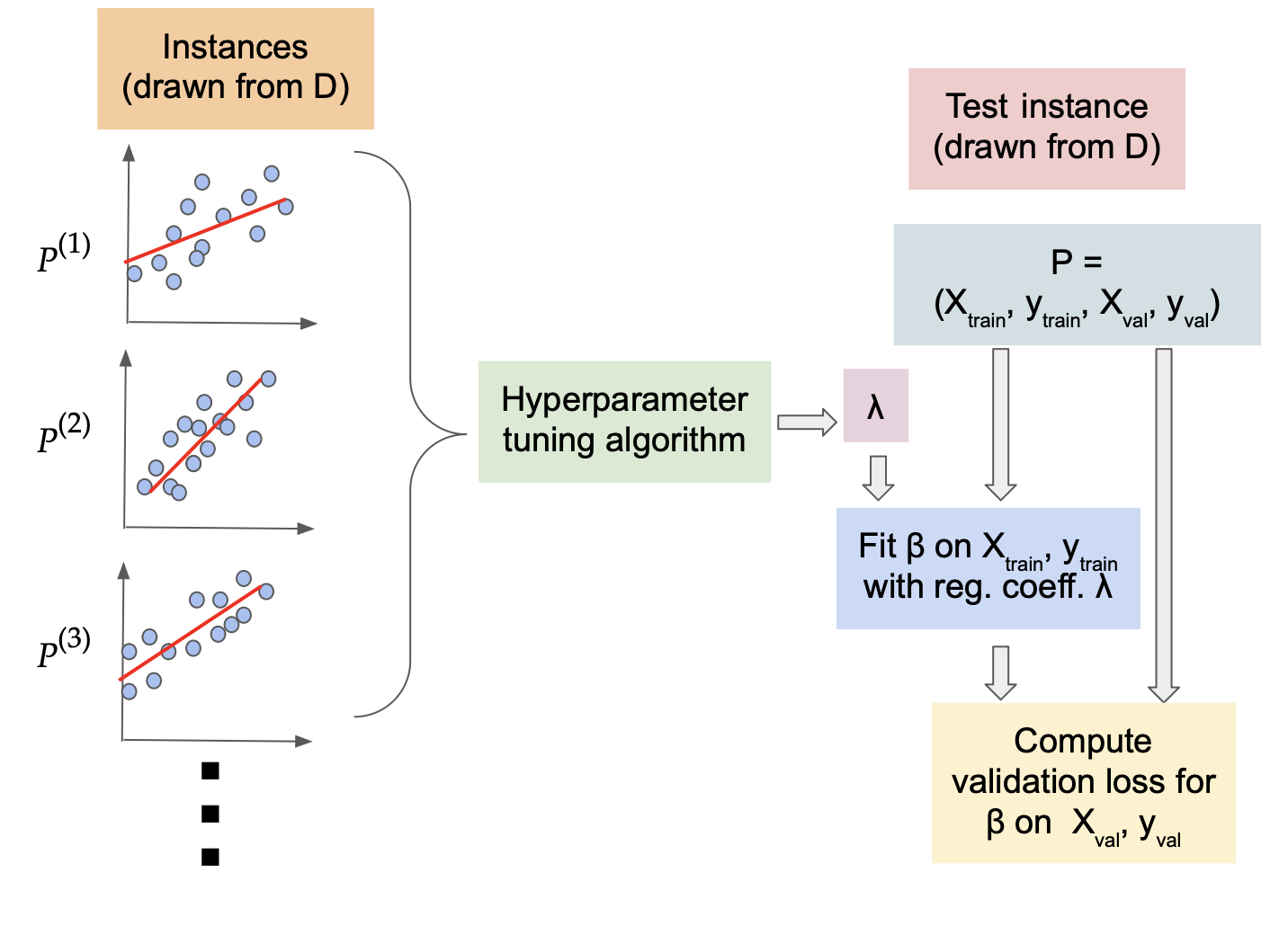
Formally, we mannequin information coming from the identical area as a hard and fast (however unknown) distribution (D) over the issue cases. To seize the well-known cross-validation setting, we take into account every downside occasion of the shape (P=(X_{textual content{prepare}}, y_{textual content{prepare}}, X_{textual content{val}}, y_{textual content{val}})). That’s, the random course of that generates the datasets and the (random or deterministic) course of that generates the splits given the information, have been mixed below (D). The aim of the educational course of is to take (N) downside samples generated from the distribution (D), and be taught regularization coefficients (hat{lambda}=(lambda_1, lambda_2)) that might generalize properly over unseen downside cases drawn from (D). That’s, on an unseen check occasion (P’=(X’_{textual content{prepare}}, y’_{textual content{prepare}}, X’_{textual content{val}}, y’_{textual content{val}})), we’ll match the mannequin (beta) utilizing the educational regularization coefficients (hat{lambda}) on (X’_{textual content{prepare}}, y’_{textual content{prepare}}), and consider the loss on the set (X’_{textual content{val}}, y’_{textual content{val}}). We search the worth of (hat{lambda}) that minimizes this loss, in expectation over the draw of the random check pattern from (D).
How a lot information do we want?
The mannequin (beta) clearly relies on each the dataset ((X,y)), and the regularization coefficients (lambda_1, lambda_2). A key device in data-driven algorithm design is the evaluation of the “twin perform”, which is the loss expressed as a perform of the parameters, for a hard and fast downside occasion. That is sometimes simpler to research than the “primal perform” (loss for a hard and fast parameter, as downside cases are diverse) in data-driven algorithm design issues. For Elastic Web regression, the twin is the validation loss on a hard and fast validation set for fashions skilled with totally different values of (lambda_1, lambda_2) (i.e. two-parameter perform) for a hard and fast coaching set. Sometimes the twin capabilities in combinatorial issues exhibit a piecewise construction, the place the habits of the loss perform can have sharp transitions throughout the items. For instance, in clustering this piecewise habits might correspond to studying a unique cluster in every bit. Prior research has proven that if we will sure the complexity of the boundary and piece capabilities within the twin perform, then we may give a pattern complexity assure, i.e. we will reply the query “how a lot information is ample to be taught an excellent worth of the parameter?”
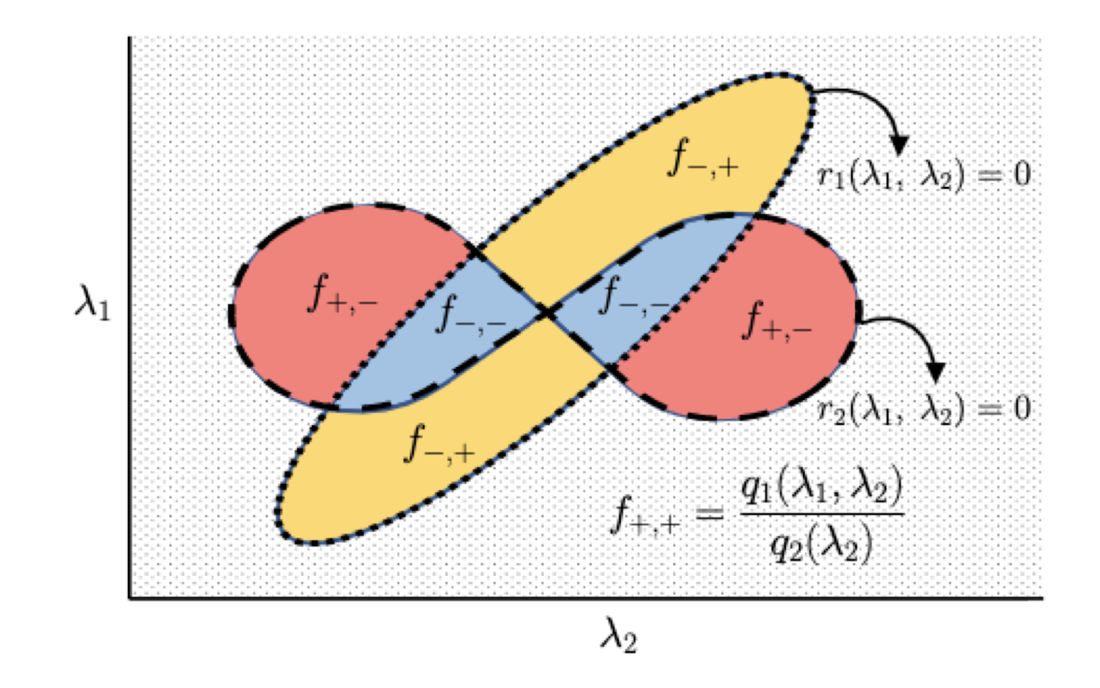
An illustration of the piecewise construction of the Elastic Web twin loss perform. Right here (r_1) and (r_2) are polynomial boundary capabilities, and (f_{*,*}) are piece capabilities that are mounted rational capabilities given the indicators of boundary capabilities.
Considerably surprisingly, we present that the twin loss perform displays a piecewise construction even in linear regression, a traditional steady optimization downside. Intuitively, the items correspond to totally different subsets of the options being “lively”, i.e. having non-zero coefficients within the realized mannequin (beta). Particularly, we present that the piece boundaries of the twin perform are polynomial capabilities of bounded diploma, and the loss inside every bit is a rational perform (ratio of two polynomial capabilities) once more of bounded diploma. We use this construction to determine a sure on the learning-theoretic complexity of the twin perform; extra exactly, we sure its pseudo-dimension (a generalization of the VC dimension to real-valued capabilities).
Theorem. The pseudo-dimension of the Elastic Web twin loss perform is (Theta(p)), the place (p) is the function dimension.
(Theta(p)) notation right here means we’ve got an higher sure of (O(p)) in addition to a decrease sure (Omega(p)) on the pseudo-dimension. Roughly talking, the pseudo-dimension captures the complexity of the perform class from a studying perspective, and corresponds to the variety of samples wanted to ensure small generalization error (common error on check information). Remarkably, we present an asymptotically tight sure on the pseudo-dimension by establishing a (Omega(p)) decrease sure which is technically difficult and wishes an express development of a set of “laborious” cases. Tight decrease bounds should not recognized for a number of typical issues in data-driven algorithm design. Our sure relies upon solely on (p) (the variety of options) and is unbiased of the variety of datapoints (m). An instantaneous consequence of our sure is the next pattern complexity assure:
Theorem. Given any distribution (D) (mounted, however unknown), we will be taught regularization parameters (hat{lambda}) which acquire error inside any (epsilon>0) of the very best parameter with chance (1-delta) utilizing solely (O(1/epsilon^2(p+log 1/delta))) downside samples.
One option to perceive our outcomes is to instantiate them within the cross-validation setting. Take into account the generally used methods of leave-one-out cross validation (LOOCV) and Monte Carlo cross validation (repeated random test-validation splits, sometimes unbiased and in a hard and fast proportion). Given a dataset of dimension (m_{textual content{tr}}), LOOCV would require (m_{textual content{tr}}) regression suits which might be computationally costly for big datasets. Alternately, we will take into account attracts from a distribution (D_{textual content{LOO}}) which generates downside cases P from a hard and fast dataset ((X, y) in R^{m+1times p} occasions R^{m+1}) by uniformly choosing (j in [m + 1]) and setting (P = (X_{−j∗}, y_{−j} , X_{j∗}, y_j )). Our outcome now implies that roughly (O(p/epsilon^2)) iterations are sufficient to find out an Elastic Web parameter (hat{lambda}) with loss inside (epsilon) (with excessive chance) of the parameter (lambda^*) obtained from operating the total LOOCV. Equally, we will outline a distribution (D_{textual content{MC}}) to seize the Monte Carlo cross validation process and decide the variety of iterations ample to get an (epsilon)-approximation of the loss corresponding parameter choice with an arbitrarily massive variety of runs. Thus, in a really exact sense, our outcomes reply the query of how a lot cross-validation is sufficient to successfully implement the above methods.
Sequential information and on-line studying
A more difficult variant of the issue assumes that the issue cases arrive sequentially, and we have to set the parameter for every occasion utilizing solely the beforehand seen cases. We will consider this as a sport between an internet adversary and the learner, the place the adversary desires to make the sequence of issues as laborious as attainable. Word that we now not assume that the issue cases are drawn from a hard and fast distribution, and this setting permits downside cases to rely on beforehand seen cases which is often extra real looking (even when there isn’t any precise adversary producing worst-case downside sequences). The learner’s aim is to carry out in addition to the very best mounted parameter in hindsight, and the distinction is known as the “remorse” of the learner.
To acquire optimistic outcomes, we make a light assumption on the smoothness of the information: we assume that the prediction values (y) are drawn from a bounded density distribution. This captures a typical information pre-processing step of including a small quantity of uniform noise to the information for mannequin stability, e.g. by setting the jitter parameter within the well-liked Python library scikit-learn. Underneath this assumption, we present additional construction on the twin loss perform. Roughly talking, we present that the placement of the piece boundaries of the twin perform throughout the issue cases don’t focus in a small area of the parameter area.This in flip implies (utilizing Balcan et al., 2018) the existence of an internet learner with common anticipated remorse (O(1/sqrt{T})), that means that we converge to the efficiency of the very best mounted parameter in hindsight because the variety of on-line rounds (T) will increase.
Extension to binary classification, together with logistic regression
Linear classifiers are additionally well-liked for the duty of binary classification, the place the (y) values are actually restricted to (0) or (1). Regularization can also be essential right here to be taught efficient fashions by avoiding overfitting and choosing vital variables. It’s notably widespread to make use of logistic regression, the place the squared loss above is changed by the logistic loss perform,
$$l_{textual content{RLR}}(beta,(X,y))=frac{1}{m}sum_{i=1}^mlog(1+exp(-y_ix_i^Tbeta)).$$
The precise loss minimization downside is considerably more difficult on this case, and it’s correspondingly troublesome to research the twin loss perform. We overcome this problem by utilizing a proxy twin perform which approximates the true loss perform, however has a less complicated piecewise construction. Roughly talking, the proxy perform considers a effective parameter grid of width (epsilon) and approximates the loss perform at every level on the grid. Moreover, it’s piecewise linear and recognized to approximate the true loss perform to inside an error of (O(epsilon^2)) in any respect factors (Rosset, 2004).
Our principal outcome for logistic regression is that the generalization error with (N) samples drawn from the distribution (D) is bounded by (O(sqrt{(m^2+log 1/epsilon)/N}+epsilon^2+sqrt{(log 1/delta)/N})), with (excessive) chance (1-delta) over the draw of samples. (m) right here is the dimensions of the validation set, which is usually small and even fixed. Whereas this sure is incomparable to the pseudo-dimension-based bounds above, we should not have decrease bounds on this setting and tightness of our leads to an fascinating open query.
Past the linear case: kernel regression
Up to now, we’ve got assumed that the dependent variable (y) has a linear dependence on the predictor variables. Whereas it is a nice very first thing to strive in lots of functions, fairly often there’s a non-linear relationship between the variables. In consequence, linear regression can lead to poor efficiency in some functions. A standard different is to make use of Kernelized Least Squares Regression, the place the enter (X) is implicitly mapped to excessive (and even infinite) dimensional function area utilizing the “kernel trick”. As a corollary of our principal outcomes, we will present that the pseudo-dimension of the twin loss perform on this case is (O(m)), the place (m) is the dimensions of the coaching set in a single downside occasion. Our outcomes don’t make any assumptions on the (m) samples inside an issue occasion/dataset; if these samples inside downside cases are additional assumed to be i.i.d. attracts from some information distribution (distinct from downside distribution (D)), then well-known results suggest that (m = O(okay log p)) samples are ample to be taught the optimum LASSO coefficient ((okay) denotes the variety of non-zero coefficients within the optimum regression match).
Some last remarks
We take into account tips on how to tune the norm-based regularization parameters in linear regression. We pin down the learning-theoretic complexity of the loss perform, which can be of unbiased curiosity. Our outcomes lengthen to on-line studying, linear classification, and kernel regression. A key path for future analysis is creating an environment friendly implementation of the algorithms underlying our method.
Extra broadly, regularization is a elementary approach in machine studying, together with deep studying the place it could possibly take the type of dropout charges, or parameters within the loss perform, with important affect on the efficiency of the general algorithm. Our analysis opens up the thrilling query of tuning learnable parameters even in steady optimization issues. Lastly, our analysis captures an more and more typical state of affairs with the arrival of the data era, the place one has entry to repeated cases of information from the identical software area.
For additional particulars about our cool outcomes and the mathematical equipment we used to derive them, take a look at our papers linked beneath!
[1] Balcan, M.-F., Khodak, M., Sharma, D., & Talwalkar, A. (2022). Provably tuning the ElasticNet across instances. Advances in Neural Data Processing Techniques, 35.
[2] Balcan, M.-F., Nguyen, A., & Sharma, D. (2023). New Bounds for Hyperparameter Tuning of Regression Problems Across Instances. Advances in Neural Data Processing Techniques, 36.