A Python Device for Fetching Air Air pollution Knowledge from Google Maps Air High quality APIs | by Robert Martin-Quick | Oct, 2023
In August 2023, Google introduced the addition of an air high quality service to its record of mapping APIs. You may learn extra about that here. It seems this info is now additionally obtainable from throughout the Google Maps app, although the information obtainable through the APIs turned out to be a lot richer.
In accordance the announcement, Google is combining info from many sources at completely different resolutions — ground-based air pollution sensors, satellite tv for pc information, stay visitors info and predictions from numerical fashions — to supply a dynamically up to date dataset of air high quality in 100 nations at as much as 500m decision. This seems like a really fascinating and probably helpful dataset for all types of mapping, healthcare and planning functions!
When first studying about this I used to be planning to attempt it out in a “speak to your information” utility, utilizing a few of the issues discovered from constructing this travel mapper software. Perhaps a system that may plot a time sequence of air air pollution concentrations in your favourite metropolis, or maybe a software to assist individuals plan hikes of their native space as to keep away from unhealthy air?
There are three API tools that may assist right here — a “present circumstances” service, which gives present air high quality index values and pollutant concentrations at a given location; a “historic circumstances” service, which does the identical however at hourly intervals for as much as 30 days prior to now and a “heatmap” service, which gives present circumstances over a given space as a picture.
Beforehand, I had used the wonderful googlemapsbundle to name Google Maps APIs in Python, however these new APIs will not be but supported. Surprisingly, past the official documentation I may discover few examples of individuals utilizing these new instruments and no pre-existing Python packages designed to name them. I might be fortunately corrected although if somebody is aware of in any other case!
I subsequently constructed some fast instruments of my very own, and on this put up we stroll via how they work and the way to use them. I hope this shall be helpful to anybody eager to experiment with these new APIs in Python and on the lookout for a spot to begin. All of the code for this venture could be discovered here, and I’ll doubtless be increasing this repo over time as I add extra performance and construct some kind of mapping utility with the air high quality information.
Let’s get began! On this part we’ll go over the way to fetch air high quality information at a given location with Google Maps. You’ll first want an API key, which you’ll be able to generate through your Google Cloud account. They’ve a 90-day free trial period, after which you’ll pay for API providers you employ. Ensure you allow the “Air High quality API”, and concentrate on the pricing insurance policies earlier than you begin making numerous calls!

I normally retailer my API key in an .env file and cargo it with dotenv utilizing a operate like this
from dotenv import load_dotenv
from pathlib import Pathdef load_secets():
load_dotenv()
env_path = Path(".") / ".env"
load_dotenv(dotenv_path=env_path)
google_maps_key = os.getenv("GOOGLE_MAPS_API_KEY")
return {
"GOOGLE_MAPS_API_KEY": google_maps_key,
}
Getting present circumstances requires a POST request as detailed here. We’re going to take inspiration from the googlemaps bundle to do that in a means that may be generalized. First, we construct a consumer class that makes use of requests to make the decision. The purpose is sort of simple — we need to construct a URL just like the one beneath, and embrace all of the request choices particular to the person’s question.
https://airquality.googleapis.com/v1/currentConditions:lookup?key=YOUR_API_KEY
The Consumerclass takes in our API key as key after which builds the request_url for the question. It accepts request choices as a params dictionary after which places them within the JSON request physique, which is dealt with by the self.session.put up() name.
import requests
import ioclass Consumer(object):
DEFAULT_BASE_URL = "https://airquality.googleapis.com"
def __init__(self, key):
self.session = requests.Session()
self.key = key
def request_post(self, url, params):
request_url = self.compose_url(url)
request_header = self.compose_header()
request_body = params
response = self.session.put up(
request_url,
headers=request_header,
json=request_body,
)
return self.get_body(response)
def compose_url(self, path):
return self.DEFAULT_BASE_URL + path + "?" + "key=" + self.key
@staticmethod
def get_body(response):
physique = response.json()
if "error" in physique:
return physique["error"]
return physique
@staticmethod
def compose_header():
return {
"Content material-Kind": "utility/json",
}
Now we are able to make a operate that helps the person assemble legitimate request choices for the present circumstances API after which makes use of this Consumer class to make the request. Once more, that is impressed by the design of the googlemaps bundle.
def current_conditions(
consumer,
location,
include_local_AQI=True,
include_health_suggestion=False,
include_all_pollutants=True,
include_additional_pollutant_info=False,
include_dominent_pollutant_conc=True,
language=None,
):
"""
See documentation for this API right here
https://builders.google.com/maps/documentation/air-quality/reference/relaxation/v1/currentConditions/lookup
"""
params = {}if isinstance(location, dict):
params["location"] = location
else:
elevate ValueError(
"Location argument should be a dictionary containing latitude and longitude"
)
extra_computations = []
if include_local_AQI:
extra_computations.append("LOCAL_AQI")
if include_health_suggestion:
extra_computations.append("HEALTH_RECOMMENDATIONS")
if include_additional_pollutant_info:
extra_computations.append("POLLUTANT_ADDITIONAL_INFO")
if include_all_pollutants:
extra_computations.append("POLLUTANT_CONCENTRATION")
if include_dominent_pollutant_conc:
extra_computations.append("DOMINANT_POLLUTANT_CONCENTRATION")
if language:
params["language"] = language
params["extraComputations"] = extra_computations
return consumer.request_post("/v1/currentConditions:lookup", params)
The choices for this API are comparatively simple. It wants a dictionary with the longitude and latitude of the purpose you need to examine, and might optionally absorb numerous different arguments that management how a lot info is returned. Lets see it in motion with all of the arguments set to True
# arrange consumer
consumer = Consumer(key=GOOGLE_MAPS_API_KEY)
# a location in Los Angeles, CA
location = {"longitude":-118.3,"latitude":34.1}
# a JSON response
current_conditions_data = current_conditions(
consumer,
location,
include_health_suggestion=True,
include_additional_pollutant_info=True
)
A number of fascinating info is returned! Not solely do we have now the air high quality index values from the Common and US-based AQI indices, however we even have concentrations of the main pollution, an outline of every one and an total set of well being suggestions for the present air high quality.
{'dateTime': '2023-10-12T05:00:00Z',
'regionCode': 'us',
'indexes': [{'code': 'uaqi',
'displayName': 'Universal AQI',
'aqi': 60,
'aqiDisplay': '60',
'color': {'red': 0.75686276, 'green': 0.90588236, 'blue': 0.09803922},
'category': 'Good air quality',
'dominantPollutant': 'pm10'},
{'code': 'usa_epa',
'displayName': 'AQI (US)',
'aqi': 39,
'aqiDisplay': '39',
'color': {'green': 0.89411765},
'category': 'Good air quality',
'dominantPollutant': 'pm10'}],
'pollution': [{'code': 'co',
'displayName': 'CO',
'fullName': 'Carbon monoxide',
'concentration': {'value': 292.61, 'units': 'PARTS_PER_BILLION'},
'additionalInfo': {'sources': 'Typically originates from incomplete combustion of carbon fuels, such as that which occurs in car engines and power plants.',
'effects': 'When inhaled, carbon monoxide can prevent the blood from carrying oxygen. Exposure may cause dizziness, nausea and headaches. Exposure to extreme concentrations can lead to loss of consciousness.'}},
{'code': 'no2',
'displayName': 'NO2',
'fullName': 'Nitrogen dioxide',
'concentration': {'value': 22.3, 'units': 'PARTS_PER_BILLION'},
'additionalInfo': {'sources': 'Main sources are fuel burning processes, such as those used in industry and transportation.',
'effects': 'Exposure may cause increased bronchial reactivity in patients with asthma, lung function decline in patients with Chronic Obstructive Pulmonary Disease (COPD), and increased risk of respiratory infections, especially in young children.'}},
{'code': 'o3',
'displayName': 'O3',
'fullName': 'Ozone',
'concentration': {'value': 24.17, 'units': 'PARTS_PER_BILLION'},
'additionalInfo': {'sources': 'Ozone is created in a chemical reaction between atmospheric oxygen, nitrogen oxides, carbon monoxide and organic compounds, in the presence of sunlight.',
'effects': 'Ozone can irritate the airways and cause coughing, a burning sensation, wheezing and shortness of breath. Additionally, ozone is one of the major components of photochemical smog.'}},
{'code': 'pm10',
'displayName': 'PM10',
'fullName': 'Inhalable particulate matter (<10µm)',
'concentration': {'value': 44.48, 'units': 'MICROGRAMS_PER_CUBIC_METER'},
'additionalInfo': {'sources': 'Main sources are combustion processes (e.g. indoor heating, wildfires), mechanical processes (e.g. construction, mineral dust, agriculture) and biological particles (e.g. pollen, bacteria, mold).',
'effects': 'Inhalable particles can penetrate into the lungs. Short term exposure can cause irritation of the airways, coughing, and aggravation of heart and lung diseases, expressed as difficulty breathing, heart attacks and even premature death.'}},
{'code': 'pm25',
'displayName': 'PM2.5',
'fullName': 'Fine particulate matter (<2.5µm)',
'concentration': {'value': 11.38, 'units': 'MICROGRAMS_PER_CUBIC_METER'},
'additionalInfo': {'sources': 'Main sources are combustion processes (e.g. power plants, indoor heating, car exhausts, wildfires), mechanical processes (e.g. construction, mineral dust) and biological particles (e.g. bacteria, viruses).',
'effects': 'Fine particles can penetrate into the lungs and bloodstream. Short term exposure can cause irritation of the airways, coughing and aggravation of heart and lung diseases, expressed as difficulty breathing, heart attacks and even premature death.'}},
{'code': 'so2',
'displayName': 'SO2',
'fullName': 'Sulfur dioxide',
'concentration': {'value': 0, 'units': 'PARTS_PER_BILLION'},
'additionalInfo': {'sources': 'Main sources are burning processes of sulfur-containing fuel in industry, transportation and power plants.',
'effects': 'Exposure causes irritation of the respiratory tract, coughing and generates local inflammatory reactions. These in turn, may cause aggravation of lung diseases, even with short term exposure.'}}],
'healthRecommendations': {'generalPopulation': 'With this stage of air high quality, you haven't any limitations. Benefit from the open air!',
'aged': 'For those who begin to really feel respiratory discomfort reminiscent of coughing or respiration difficulties, contemplate decreasing the depth of your out of doors actions. Attempt to restrict the time you spend close to busy roads, development websites, open fires and different sources of smoke.',
'lungDiseasePopulation': 'For those who begin to really feel respiratory discomfort reminiscent of coughing or respiration difficulties, contemplate decreasing the depth of your out of doors actions. Attempt to restrict the time you spend close to busy roads, industrial emission stacks, open fires and different sources of smoke.',
'heartDiseasePopulation': 'For those who begin to really feel respiratory discomfort reminiscent of coughing or respiration difficulties, contemplate decreasing the depth of your out of doors actions. Attempt to restrict the time you spend close to busy roads, development websites, industrial emission stacks, open fires and different sources of smoke.',
'athletes': 'For those who begin to really feel respiratory discomfort reminiscent of coughing or respiration difficulties, contemplate decreasing the depth of your out of doors actions. Attempt to restrict the time you spend close to busy roads, development websites, industrial emission stacks, open fires and different sources of smoke.',
'pregnantWomen': 'To maintain you and your child wholesome, contemplate decreasing the depth of your out of doors actions. Attempt to restrict the time you spend close to busy roads, development websites, open fires and different sources of smoke.',
'youngsters': 'For those who begin to really feel respiratory discomfort reminiscent of coughing or respiration difficulties, contemplate decreasing the depth of your out of doors actions. Attempt to restrict the time you spend close to busy roads, development websites, open fires and different sources of smoke.'}}
Wouldn’t or not it’s good to have the ability to fetch a timeseries of those AQI and pollutant values for a given location? Which may reveal fascinating patterns reminiscent of correlations between the pollution or day by day fluctuations brought on by visitors or weather-related elements.
We will do that with one other POST request to the historical conditions API, which can give us an hourly historical past. This works in a lot the identical means as present circumstances, the one main distinction being that because the outcomes could be fairly lengthy they’re returned as a number of pages , which requires slightly additional logic to deal with.
Let’s modify the request_post technique of Consumer to deal with this.
def request_post(self,url,params):request_url = self.compose_url(url)
request_header = self.compose_header()
request_body = params
response = self.session.put up(
request_url,
headers=request_header,
json=request_body,
)
response_body = self.get_body(response)
# put the primary web page within the response dictionary
web page = 1
final_response = {
"page_{}".format(web page) : response_body
}
# fetch all of the pages if wanted
whereas "nextPageToken" in response_body:
# name once more with the following web page's token
request_body.replace({
"pageToken":response_body["nextPageToken"]
})
response = self.session.put up(
request_url,
headers=request_header,
json=request_body,
)
response_body = self.get_body(response)
web page += 1
final_response["page_{}".format(page)] = response_body
return final_response
This handles the case the place response_body comprises a area referred to as nextPageToken, which is the id of the following web page of knowledge that’s been generated and is able to fetch. The place that info exists, we simply must name the API once more with a brand new param referred to as pageToken , which directs it to the related web page. We do that repeatedly shortly loop till there aren’t any extra pages left. Our final_response dictionary subsequently now comprises one other layer denoted by web page quantity. For calls to current_conditions there’ll solely ever be one web page, however for calls to historical_conditions there could also be a number of.
With that taken care of, we are able to write a historical_conditions operate in a really comparable type to current_conditions .
def historical_conditions(
consumer,
location,
specific_time=None,
lag_time=None,
specific_period=None,
include_local_AQI=True,
include_health_suggestion=False,
include_all_pollutants=True,
include_additional_pollutant_info=False,
include_dominant_pollutant_conc=True,
language=None,
):
"""
See documentation for this API right here https://builders.google.com/maps/documentation/air-quality/reference/relaxation/v1/historical past/lookup
"""
params = {}if isinstance(location, dict):
params["location"] = location
else:
elevate ValueError(
"Location argument should be a dictionary containing latitude and longitude"
)
if isinstance(specific_period, dict) and never specific_time and never lag_time:
assert "startTime" in specific_period
assert "endTime" in specific_period
params["period"] = specific_period
elif specific_time and never lag_time and never isinstance(specific_period, dict):
# word that point should be within the "Zulu" format
# e.g. datetime.datetime.strftime(datetime.datetime.now(),"%Y-%m-%dTpercentH:%M:%SZ")
params["dateTime"] = specific_time
# lag durations in hours
elif lag_time and never specific_time and never isinstance(specific_period, dict):
params["hours"] = lag_time
else:
elevate ValueError(
"Should present specific_time, specific_period or lag_time arguments"
)
extra_computations = []
if include_local_AQI:
extra_computations.append("LOCAL_AQI")
if include_health_suggestion:
extra_computations.append("HEALTH_RECOMMENDATIONS")
if include_additional_pollutant_info:
extra_computations.append("POLLUTANT_ADDITIONAL_INFO")
if include_all_pollutants:
extra_computations.append("POLLUTANT_CONCENTRATION")
if include_dominant_pollutant_conc:
extra_computations.append("DOMINANT_POLLUTANT_CONCENTRATION")
if language:
params["language"] = language
params["extraComputations"] = extra_computations
# web page dimension default set to 100 right here
params["pageSize"] = 100
# web page token will get stuffed in if wanted by the request_post technique
params["pageToken"] = ""
return consumer.request_post("/v1/historical past:lookup", params)
To outline the historic interval, the API can settle for a lag_time in hours, as much as 720 (30 days). It could additionally settle for a specific_perioddictionary, with defines begin and finish instances within the format described within the feedback above. Lastly, to fetch a single hour of knowledge, it could actually settle for only one timestamp, offered by specific_time . Additionally word using the pageSize parameter, which controls what number of time factors are returned in every name to the API. The default right here is 100.
Let’s attempt it out.
# arrange consumer
consumer = Consumer(key=GOOGLE_MAPS_API_KEY)
# a location in Los Angeles, CA
location = {"longitude":-118.3,"latitude":34.1}
# a JSON response
history_conditions_data = historical_conditions(
consumer,
location,
lag_time=720
)
We should always get an extended, nested JSON response that comprises the AQI index values and particular pollutant values at 1 hour increments during the last 720 hours. There are lots of methods to format this right into a construction that’s extra amenable to visualization and evaluation, and the operate beneath will convert it right into a pandas dataframe in “lengthy” format, which works properly with seabornfor plotting.
from itertools import chain
import pandas as pddef historical_conditions_to_df(response_dict):
chained_pages = record(chain(*[response_dict[p]["hoursInfo"] for p in [*response_dict]]))
all_indexes = []
all_pollutants = []
for i in vary(len(chained_pages)):
# want this test in case one of many timestamps is lacking information, which may typically occur
if "indexes" in chained_pages[i]:
this_element = chained_pages[i]
# fetch the time
time = this_element["dateTime"]
# fetch all of the index values and add metadata
all_indexes += [(time , x["code"],x["displayName"],"index",x["aqi"],None) for x in this_element['indexes']]
# fetch all of the pollutant values and add metadata
all_pollutants += [(time , x["code"],x["fullName"],"pollutant",x["concentration"]["value"],x["concentration"]["units"]) for x in this_element['pollutants']]
all_results = all_indexes + all_pollutants
# generate "lengthy format" dataframe
res = pd.DataFrame(all_results,columns=["time","code","name","type","value","unit"])
res["time"]=pd.to_datetime(res["time"])
return res
Operating this on the output of historical_conditions will produce a dataframe whose columns are formatted for simple evaluation.
df = historical_conditions_to_df(history_conditions_data)

And we are able to now plot the lead to seaborn or another visualization software.
import seaborn as sns
g = sns.relplot(
x="time",
y="worth",
information=df[df["code"].isin(["uaqi","usa_epa","pm25","pm10"])],
type="line",
col="identify",
col_wrap=4,
hue="kind",
peak=4,
facet_kws={'sharey': False, 'sharex': False}
)
g.set_xticklabels(rotation=90)

That is already very fascinating! There are clearly a number of periodicities within the pollutant time sequence and it’s notable that the US AQI is carefully correlated with the pm25 and pm10 concentrations, as anticipated. I’m a lot much less acquainted with the Common AQI that Google is offering right here, so can’t clarify why seems anti-correlated with pm25 and p10. Does smaller UAQI imply higher air high quality? Regardless of some looking out round I’ve been unable to discover a good reply.
Now for the ultimate use case of the Google Maps Air High quality API — producing heatmap tiles. The documentation about this a sparse, which is a disgrace as a result of these tiles are a robust software for visualizing present air high quality, particularly when mixed with a Folium map.
We fetch them with a GET request, which includes constructing a URL within the following format, the place the placement of the tile is specified by zoom , x and y
GET https://airquality.googleapis.com/v1/mapTypes/{mapType}/heatmapTiles/{zoom}/{x}/{y}
What dozoom , x and y imply? We will answe this by studying about how Google Maps converts coordinates in latitude and longitude into “tile coordinates”, which is described intimately here. Primarily, Google Maps is storing imagery in grids the place every cell measures 256 x 256 pixels and the real-world dimensions of the cell are a operate of the zoom stage. After we make a name to the API, we have to specify which grid to attract from — which is set by the zoom stage — and the place on the grid to attract from — which is set by the x and y tile coordinates. What comes again is a bytes array that may be learn by Python Imaging Library (PIL) or similiar imaging processing bundle.
Having fashioned our url within the above format, we are able to add just a few strategies to the Consumer class that can enable us to fetch the corresponding picture.
def request_get(self,url):request_url = self.compose_url(url)
response = self.session.get(request_url)
# for pictures coming from the heatmap tiles service
return self.get_image(response)
@staticmethod
def get_image(response):
if response.status_code == 200:
image_content = response.content material
# word use of Picture from PIL right here
# wants from PIL import Picture
picture = Picture.open(io.BytesIO(image_content))
return picture
else:
print("GET request for picture returned an error")
return None
That is good, however we what we actually want is the power to transform a set of coordinates in longitude and latitude into tile coordinates. The documentation explains how — we first convert to coordinates into the Mercator projection, from which we convert to “pixel coordinates” utilizing the desired zoom stage. Lastly we translate that into the tile coordinates. To deal with all these transformations, we are able to use the TileHelper class beneath.
import math
import numpy as npclass TileHelper(object):
def __init__(self, tile_size=256):
self.tile_size = tile_size
def location_to_tile_xy(self,location,zoom_level=4):
# Primarily based on operate right here
# https://builders.google.com/maps/documentation/javascript/examples/map-coordinates#maps_map_coordinates-javascript
lat = location["latitude"]
lon = location["longitude"]
world_coordinate = self._project(lat,lon)
scale = 1 << zoom_level
pixel_coord = (math.flooring(world_coordinate[0]*scale), math.flooring(world_coordinate[1]*scale))
tile_coord = (math.flooring(world_coordinate[0]*scale/self.tile_size),math.flooring(world_coordinate[1]*scale/self.tile_size))
return world_coordinate, pixel_coord, tile_coord
def tile_to_bounding_box(self,tx,ty,zoom_level):
# see https://builders.google.com/maps/documentation/javascript/coordinates
# for particulars
box_north = self._tiletolat(ty,zoom_level)
# tile numbers advance in the direction of the south
box_south = self._tiletolat(ty+1,zoom_level)
box_west = self._tiletolon(tx,zoom_level)
# time numbers advance in the direction of the east
box_east = self._tiletolon(tx+1,zoom_level)
# (latmin, latmax, lonmin, lonmax)
return (box_south, box_north, box_west, box_east)
@staticmethod
def _tiletolon(x,zoom):
return x / math.pow(2.0,zoom) * 360.0 - 180.0
@staticmethod
def _tiletolat(y,zoom):
n = math.pi - (2.0 * math.pi * y)/math.pow(2.0,zoom)
return math.atan(math.sinh(n))*(180.0/math.pi)
def _project(self,lat,lon):
siny = math.sin(lat*math.pi/180.0)
siny = min(max(siny,-0.9999), 0.9999)
return (self.tile_size*(0.5 + lon/360), self.tile_size*(0.5 - math.log((1 + siny) / (1 - siny)) / (4 * math.pi)))
@staticmethod
def find_nearest_corner(location,bounds):
corner_lat_idx = np.argmin([
np.abs(bounds[0]-location["latitude"]),
np.abs(bounds[1]-location["latitude"])
])
corner_lon_idx = np.argmin([
np.abs(bounds[2]-location["longitude"]),
np.abs(bounds[3]-location["longitude"])
])
if (corner_lat_idx == 0) and (corner_lon_idx == 0):
# closests is latmin, lonmin
path = "southwest"
elif (corner_lat_idx == 0) and (corner_lon_idx == 1):
path = "southeast"
elif (corner_lat_idx == 1) and (corner_lon_idx == 0):
path = "northwest"
else:
path = "northeast"
corner_coords = (bounds[corner_lat_idx],bounds[corner_lon_idx+2])
return corner_coords, path
@staticmethod
def get_ajoining_tiles(tx,ty,path):
if path == "southwest":
return [(tx-1,ty),(tx-1,ty+1),(tx,ty+1)]
elif path == "southeast":
return [(tx+1,ty),(tx+1,ty-1),(tx,ty-1)]
elif path == "northwest":
return [(tx-1,ty-1),(tx-1,ty),(tx,ty-1)]
else:
return [(tx+1,ty-1),(tx+1,ty),(tx,ty-1)]
We will see that location_to_tile_xy is taking in a location dictionary and zoom stage and returning the tile by which that time could be discovered. One other useful operate is tile_to_bounding_box , which can discover the bounding coordinates of a specified grid cell. We want this if we’re going to geolocate the cell and plot it on a map.
Lets see how this works contained in the air_quality_tile operate beneath, which goes to absorb our consumer , location and a string indicating what kind of tile we need to fetch. We additionally must specify a zoom stage, which could be troublesome to decide on at first and requires some trial and error. We’ll focus on the get_adjoining_tiles argument shortly.
def air_quality_tile(
consumer,
location,
pollutant="UAQI_INDIGO_PERSIAN",
zoom=4,
get_adjoining_tiles = True):
# see https://builders.google.com/maps/documentation/air-quality/reference/relaxation/v1/mapTypes.heatmapTiles/lookupHeatmapTile
assert pollutant in [
"UAQI_INDIGO_PERSIAN",
"UAQI_RED_GREEN",
"PM25_INDIGO_PERSIAN",
"GBR_DEFRA",
"DEU_UBA",
"CAN_EC",
"FRA_ATMO",
"US_AQI"
]
# comprises helpful strategies for dealing the tile coordinates
helper = TileHelper()
# get the tile that the placement is in
world_coordinate, pixel_coord, tile_coord = helper.location_to_tile_xy(location,zoom_level=zoom)
# get the bounding field of the tile
bounding_box = helper.tile_to_bounding_box(tx=tile_coord[0],ty=tile_coord[1],zoom_level=zoom)
if get_adjoining_tiles:
nearest_corner, nearest_corner_direction = helper.find_nearest_corner(location, bounding_box)
adjoining_tiles = helper.get_ajoining_tiles(tile_coord[0],tile_coord[1],nearest_corner_direction)
else:
adjoining_tiles = []
tiles = []
#get all of the adjoining tiles, plus the one in query
for tile in adjoining_tiles + [tile_coord]:
bounding_box = helper.tile_to_bounding_box(tx=tile[0],ty=tile[1],zoom_level=zoom)
image_response = consumer.request_get(
"/v1/mapTypes/" + pollutant + "/heatmapTiles/" + str(zoom) + '/' + str(tile[0]) + '/' + str(tile[1])
)
# convert the PIL picture to numpy
attempt:
image_response = np.array(image_response)
besides:
image_response = None
tiles.append({
"bounds":bounding_box,
"picture":image_response
})
return tiles
From studying the code, we are able to see that the workflow is as follows: First, discover the tile coordinates of the placement of curiosity. This specifies the grid cell we need to fetch. Then, discover the bounding coordinates of this grid cell. If we need to fetch the encircling tiles, discover the closest nook of the bounding field after which use that to calculate the tile coordinates of the three adjoining grid cells. Then name the API and return every of the tiles as a picture with its corresponding bounding field.
We will run this in the usual means, as follows:
consumer = Consumer(key=GOOGLE_MAPS_API_KEY)
location = {"longitude":-118.3,"latitude":34.1}
zoom = 7
tiles = air_quality_tile(
consumer,
location,
pollutant="UAQI_INDIGO_PERSIAN",
zoom=zoom,
get_adjoining_tiles=False)
After which plot with folium for a zoomable map! Notice that I’m utilizing leafmap right here, as a result of this bundle can generate Folium maps which are appropriate with gradio, a robust software for producing easy person interfaces for python functions. Check out this article for an instance.
import leafmap.foliumap as leafmap
import foliumlat = location["latitude"]
lon = location["longitude"]
map = leafmap.Map(location=[lat, lon], tiles="OpenStreetMap", zoom_start=zoom)
for tile in tiles:
latmin, latmax, lonmin, lonmax = tile["bounds"]
AQ_image = tile["image"]
folium.raster_layers.ImageOverlay(
picture=AQ_image,
bounds=[[latmin, lonmin], [latmax, lonmax]],
opacity=0.7
).add_to(map)
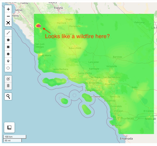
Maybe disappointingly, the tile containing our location at this zoom stage is generally sea, though its nonetheless good to see the air air pollution plotted on prime of an in depth map. For those who zoom in, you’ll be able to see that highway visitors info is getting used to tell the air high quality alerts in city areas.

Setting get_adjoining_tiles=True provides us a a lot nicer map as a result of it fetches the three closest, non-overlapping tiles at that zoom stage. In our case that helps rather a lot to make the map extra presentable.

I personally choose the photographs generated when pollutant=US_AQI, however there are a number of completely different choices. Sadly the API doesn’t return a colour scale, though it could be doable to generate one utilizing the pixel values within the picture and data of what the colours imply.

Thanks for making it to the top! Right here we explored the way to use the Google Maps Air High quality APIs to ship leads to Python, which might be utilized in method of fascinating functions. In future I hope to observe up with one other article in regards to the air_quality_mapper software because it evolves additional, however I hope that the scripts mentioned right here shall be helpful in their very own proper. As all the time, any recommendations for additional improvement can be a lot appreciated!


