Construct a crop segmentation machine studying mannequin with Planet knowledge and Amazon SageMaker geospatial capabilities

This visitor submit is co-written by Lydia Lihui Zhang, Enterprise Growth Specialist, and Mansi Shah, Software program Engineer/Knowledge Scientist, at Planet Labs. The analysis that inspired this post was initially written by Jennifer Reiber Kyle.

Amazon SageMaker geospatial capabilities mixed with Planet’s satellite tv for pc knowledge can be utilized for crop segmentation, and there are quite a few purposes and potential advantages of this evaluation to the fields of agriculture and sustainability. In late 2023, Planet announced a partnership with AWS to make its geospatial knowledge accessible by means of Amazon SageMaker.

Crop segmentation is the method of splitting up a satellite tv for pc picture into areas of pixels, or segments, which have comparable crop traits. On this submit, we illustrate use a segmentation machine studying (ML) mannequin to establish crop and non-crop areas in a picture.

Figuring out crop areas is a core step in the direction of gaining agricultural insights, and the mixture of wealthy geospatial knowledge and ML can result in insights that drive choices and actions. For instance:

• Making data-driven farming choices – By gaining higher spatial understanding of the crops, farmers and different agricultural stakeholders can optimize using assets, from water to fertilizer to different chemical substances throughout the season. This units the muse for decreasing waste, bettering sustainable farming practices wherever attainable, and growing productiveness whereas minimizing environmental impression.
• Figuring out climate-related stresses and developments – As local weather change continues to have an effect on world temperature and rainfall patterns, crop segmentation can be utilized to establish areas which are weak to climate-related stress for local weather adaptation methods. For instance, satellite tv for pc imagery archives can be utilized to trace modifications in a crop rising area over time. These might be the bodily modifications in dimension and distribution of croplands. They may be the modifications in soil moisture, soil temperature, and biomass, derived from the totally different spectral index of satellite tv for pc knowledge, for deeper crop well being evaluation.
• Assessing and mitigating harm – Lastly, crop segmentation can be utilized to rapidly and precisely establish areas of crop harm within the occasion of a pure catastrophe, which will help prioritize aid efforts. For instance, after a flood, high-cadence satellite tv for pc photos can be utilized to establish areas the place crops have been submerged or destroyed, permitting aid organizations to help affected farmers extra rapidly.

On this evaluation, we use a Ok-nearest neighbors (KNN) mannequin to conduct crop segmentation, and we examine these outcomes with floor fact imagery on an agricultural area. Our outcomes reveal that the classification from the KNN mannequin is extra precisely consultant of the state of the present crop area in 2017 than the bottom fact classification knowledge from 2015. These outcomes are a testomony to the facility of Planet’s high-cadence geospatial imagery. Agricultural fields change typically, typically a number of occasions a season, and having high-frequency satellite tv for pc imagery accessible to look at and analyze this land can present immense worth to our understanding of agricultural land and quickly-changing environments.

Planet and AWS’s partnership on geospatial ML

SageMaker geospatial capabilities empower knowledge scientists and ML engineers to construct, practice, and deploy fashions utilizing geospatial knowledge. SageMaker geospatial capabilities help you effectively remodel or enrich large-scale geospatial datasets, speed up mannequin constructing with pre-trained ML fashions, and discover mannequin predictions and geospatial knowledge on an interactive map utilizing 3D-accelerated graphics and built-in visualization instruments. With SageMaker geospatial capabilities, you possibly can course of massive datasets of satellite tv for pc imagery and different geospatial knowledge to create correct ML fashions for numerous purposes, together with crop segmentation, which we talk about on this submit.

Planet Labs PBC is a number one Earth-imaging firm that makes use of its massive fleet of satellites to seize imagery of the Earth’s floor every day. Planet’s knowledge is due to this fact a precious useful resource for geospatial ML. Its high-resolution satellite tv for pc imagery can be utilized to establish numerous crop traits and their well being over time, wherever on Earth.

The partnership between Planet and SageMaker permits clients to simply entry and analyze Planet’s high-frequency satellite tv for pc knowledge utilizing AWS’s highly effective ML instruments. Knowledge scientists can carry their very own knowledge or conveniently discover and subscribe to Planet’s knowledge with out switching environments.

Crop segmentation in an Amazon SageMaker Studio pocket book with a geospatial picture

On this instance geospatial ML workflow, we have a look at carry Planet’s knowledge together with the bottom fact knowledge supply into SageMaker, and practice, infer, and deploy a crop segmentation mannequin with a KNN classifier. Lastly, we assess the accuracy of our outcomes and examine this to our floor fact classification.

The KNN classifier used was educated in an Amazon SageMaker Studio notebook with a geospatial picture, and offers a versatile and extensible pocket book kernel for working with geospatial knowledge.

The Amazon SageMaker Studio pocket book with geospatial picture comes pre-installed with generally used geospatial libraries similar to GDAL, Fiona, GeoPandas, Shapely, and Rasterio, which permit the visualization and processing of geospatial knowledge instantly inside a Python pocket book setting. Widespread ML libraries similar to OpenCV or scikit-learn are additionally used to carry out crop segmentation utilizing KNN classification, and these are additionally put in within the geospatial kernel.

Knowledge choice

The agricultural area we zoom into is situated on the often sunny Sacramento County in California.

Why Sacramento? The realm and time choice for this kind of downside is primarily outlined by the supply of floor fact knowledge, and such knowledge in crop kind and boundary knowledge, will not be simple to return by. The 2015 Sacramento County Land Use DWR Survey dataset is a publicly accessible dataset masking Sacramento County in that yr and offers hand-adjusted boundaries.

The first satellite tv for pc imagery we use is the Planet’s 4-band PSScene Product, which accommodates the Blue, Inexperienced, Crimson, and Close to-IR bands and is radiometrically corrected to at-sensor radiance. The coefficients for correcting to at-sensor reflectance are offered within the scene metadata, which additional improves the consistency between photos taken at totally different occasions.

Planet’s Dove satellites that produced this imagery have been launched February 14, 2017 (news release), due to this fact they didn’t picture Sacramento County again in 2015. Nonetheless, they’ve been taking day by day imagery of the realm for the reason that launch. On this instance, we accept the imperfect 2-year hole between the bottom fact knowledge and satellite tv for pc imagery. Nonetheless, Landsat 8 lower-resolution imagery might have been used as a bridge between 2015 and 2017.

Entry Planet knowledge

To assist customers get correct and actionable knowledge quicker, Planet has additionally developed the Planet Software program Growth Equipment (SDK) for Python. It is a highly effective instrument for knowledge scientists and builders who wish to work with satellite tv for pc imagery and different geospatial knowledge. With this SDK, you possibly can search and entry Planet’s huge assortment of high-resolution satellite tv for pc imagery, in addition to knowledge from different sources like OpenStreetMap. The SDK offers a Python shopper to Planet’s APIs, in addition to a no-code command line interface (CLI) answer, making it simple to include satellite tv for pc imagery and geospatial knowledge into Python workflows. This instance makes use of the Python shopper to establish and obtain imagery wanted for the evaluation.

You may set up the Planet Python shopper within the SageMaker Studio pocket book with geospatial picture utilizing a easy command:

You should use the shopper to question related satellite tv for pc imagery and retrieve a listing of obtainable outcomes primarily based on the realm of curiosity, time vary, and different search standards. Within the following instance, we begin by asking what number of PlanetScope scenes (Planet’s day by day imagery) cowl the identical space of curiosity (AOI) that we outline earlier by means of the bottom knowledge in Sacramento, given a sure time vary between June 1 and October 1, 2017; in addition to a sure desired most cloud protection vary of 10%:

# create a request utilizing the SDK from the search specs of the info

item_type = ['PSScene']

geom_filter_train = data_filter.geometry_filter(aoi_train)
date_range_filter = data_filter.date_range_filter("acquired", gt=datetime(month=6, day=1, yr=2017), lt=datetime(month=10, day=1, yr=2017))
cloud_cover_filter = data_filter.range_filter('cloud_cover', lt=0.10)

combined_filter_test = data_filter.and_filter([geom_filter_test, date_range_filter, cloud_cover_filter])
    
# Run a fast seek for our TRAIN knowledge
async with Session() as sess:
    cl = sess.shopper('knowledge')
    outcomes = cl.search(title="temp_search_train",search_filter=combined_filter_train, item_types=item_type)
    train_result_list = [i async for i in results]

print("Variety of practice scene outcomes: ", len(train_result_list))

The returned outcomes present the variety of matching scenes overlapping with our space of curiosity. It additionally accommodates every scene’s metadata, its picture ID, and a preview picture reference.

After a selected scene has been chosen, with specification on the scene ID, merchandise kind, and product bundles (reference documentation), you need to use the next code to obtain the picture and its metadata:

train_scene_id = '20170601_180425_0f35'
item_type="PSScene"
bundle_type="analytic_sr_udm2"

# outline the order request
merchandise = [order_request.product([train_scene_id], bundle_type, item_type)]
request = order_request.build_request('train_dataset', merchandise=merchandise)

# obtain the coaching knowledge
async with Session() as sess:
    cl = sess.shopper('orders')
    # use "reporting" to handle polling for order standing
    with reporting.StateBar(state="creating") as bar:
        # carry out the order with the prior created order request
        order = await cl.create_order(request)
        bar.replace(state="created", order_id=train_order['id'])

        # wait by way of polling till the order is processed
        await cl.wait(train_order['id'], callback=bar.update_state)

    #  obtain the precise asset
    await cl.download_order(order_id=order['id'], listing=download_directory, progress_bar=True, overwrite=True)

This code downloads the corresponding satellite tv for pc picture to the Amazon Elastic File System (Amazon EFS) quantity for SageMaker Studio.

Mannequin coaching

After the info has been downloaded with the Planet Python shopper, the segmentation mannequin may be educated. On this instance, a mixture of KNN classification and picture segmentation strategies is used to establish crop space and create georeferenced geojson options.

The Planet knowledge is loaded and preprocessed utilizing the built-in geospatial libraries and instruments in SageMaker to arrange it for coaching the KNN classifier. The bottom fact knowledge for coaching is the Sacramento County Land Use DWR Survey dataset from 2015, and the Planet knowledge from 2017 is used for testing the mannequin.

Convert floor fact options to contours

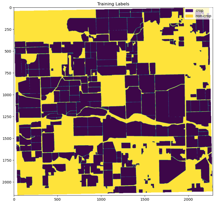
To coach the KNN classifier, the category of every pixel as both crop or non-crop must be recognized. The category is set by whether or not the pixel is related to a crop function within the floor fact knowledge or not. To make this dedication, the bottom fact knowledge is first transformed into OpenCV contours, that are then used to separate crop from non-crop pixels. The pixel values and their classification are then used to coach the KNN classifier.

To transform the bottom fact options to contours, the options should first be projected to the coordinate reference system of the picture. Then, the options are remodeled into picture area, and eventually transformed into contours. To make sure the accuracy of the contours, they’re visualized overlaid on the enter picture, as proven within the following instance.

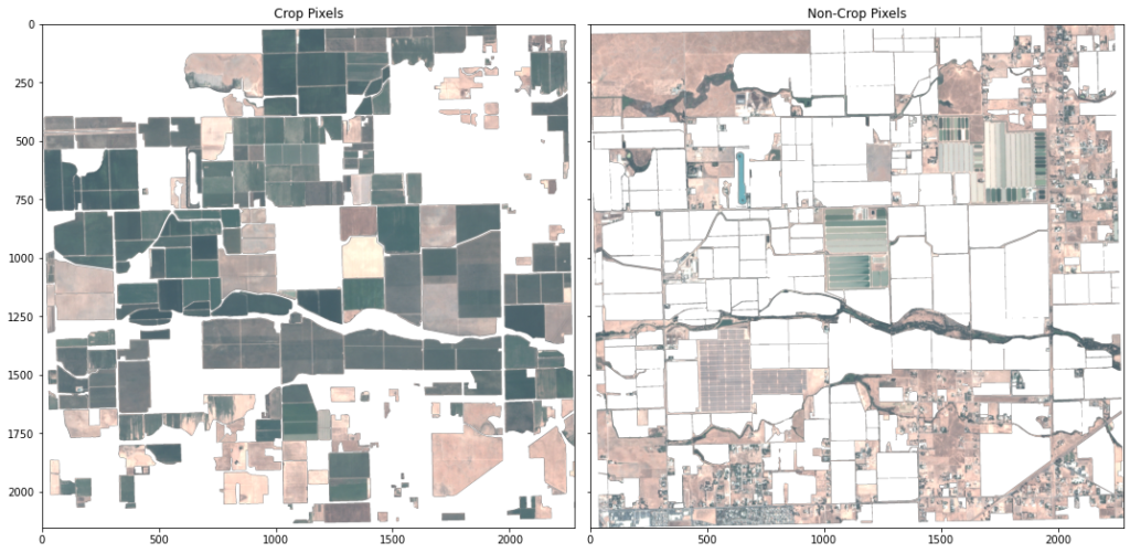
To coach the KNN classifier, crop and non-crop pixels are separated utilizing the crop function contours as a masks.

The enter of KNN classifier consists of two datasets: X, a 2nd array that gives the options to be categorised on; and y, a 1d array that gives the courses (example). Right here, a single categorised band is created from the non-crop and crop datasets, the place the band’s values point out the pixel class. The band and the underlying picture pixel band values are then transformed to the X and y inputs for the classifier match operate.

Practice the classifier on crop and non-crop pixels

The KNN classification is carried out with the scikit-learn KNeighborsClassifier. The variety of neighbors, a parameter significantly affecting the estimator’s efficiency, is tuned utilizing cross-validation in KNN cross-validation. The classifier is then educated utilizing the ready datasets and the tuned variety of neighbor parameters. See the next code:

def fit_classifier(pl_filename, ground_truth_filename, metadata_filename, n_neighbors):
    weights="uniform"
    clf = neighbors.KNeighborsClassifier(n_neighbors, weights=weights)
    train_class_band = create_contour_classified_band(pl_filename, ground_truth_filename)
    X = to_X(load_refl_bands(pl_filename, metadata_filename))
    y = to_y(train_class_band)
    clf.match(X, y)
    return clf

clf = fit_classifier(train_scene_filename,
                     train_ground_truth_filename,
                     train_metadata_filename,
                     n_neighbors)

To evaluate the classifier’s efficiency on its enter knowledge, the pixel class is predicted utilizing the pixel band values. The classifier’s efficiency is principally primarily based on the accuracy of the coaching knowledge and the clear separation of the pixel courses primarily based on the enter knowledge (pixel band values). The classifier’s parameters, such because the variety of neighbors and the gap weighting operate, may be adjusted to compensate for any inaccuracies within the latter. See the next code:

def predict(pl_filename, metadata_filename, clf):
    bands = load_refl_bands(pl_filename, metadata_filename)
    X = to_X(bands)
    y = clf.predict(X)
    return classified_band_from_y(bands[0].masks, y)

train_predicted_class_band = predict(train_scene_filename, train_metadata_filename, clf)

Consider mannequin predictions

The educated KNN classifier is utilized to foretell crop areas within the check knowledge. This check knowledge consists of areas that weren’t uncovered to the mannequin throughout coaching. In different phrases, the mannequin has no data of the realm previous to its evaluation and due to this fact this knowledge can be utilized to objectively consider the mannequin’s efficiency. We begin by visually inspecting a number of areas, starting with a area that’s comparatively noisier.

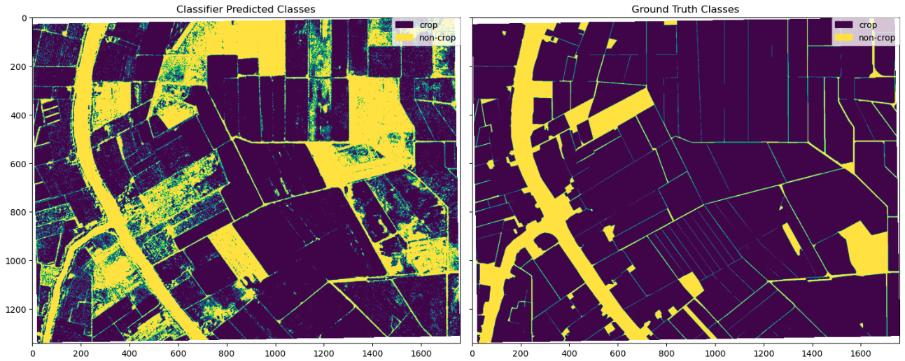
The visible inspection reveals that the anticipated courses are largely in line with the bottom fact courses. There are just a few areas of deviation, which we examine additional.

Upon additional investigation, we found that among the noise on this area was because of the floor fact knowledge missing the element that’s current within the categorised picture (high proper in comparison with high left and backside left). A very attention-grabbing discovering is that the classifier identifies bushes alongside the river as non-crop, whereas the bottom fact knowledge mistakenly identifies them as crop. This distinction between these two segmentations could also be because of the bushes shading the area over the crops.

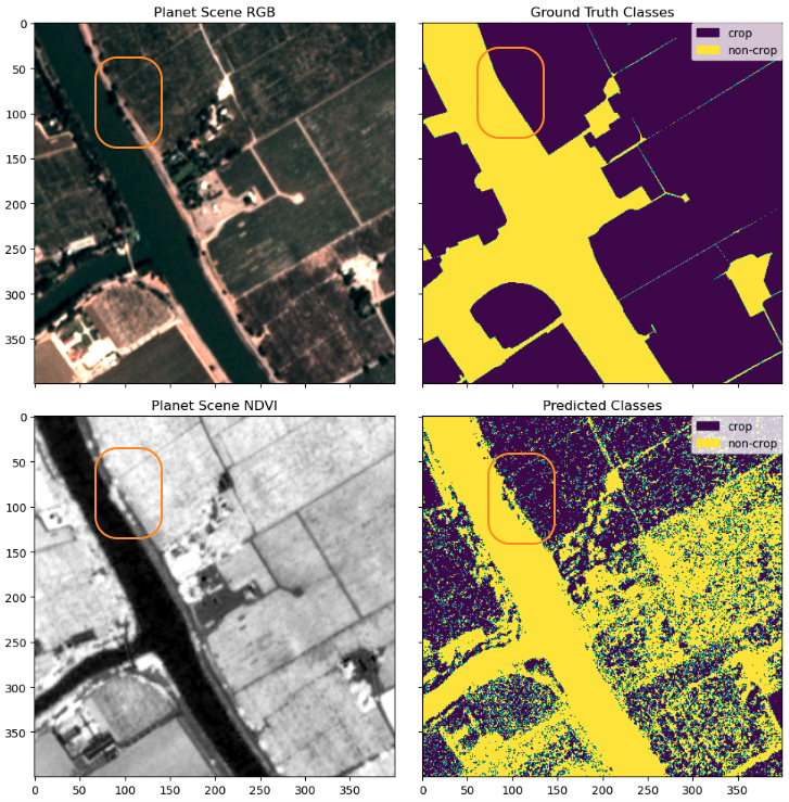
Following this, we examine one other area that was categorised in a different way between the 2 strategies. These highlighted areas have been beforehand marked as non-crop areas within the floor fact knowledge in 2015 (high proper) however modified and proven clearly as cropland in 2017 by means of the Planetscope Scenes (high left and backside left). They have been additionally categorised largely as cropland by means of the classifier (backside proper).

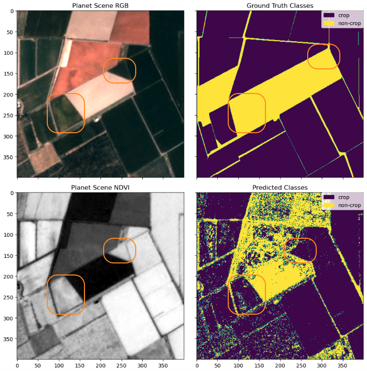
Once more, we see the KNN classifier presents a extra granular end result than the bottom fact class, and it additionally efficiently captures the change taking place within the cropland. This instance additionally speaks to the worth of day by day refreshed satellite tv for pc knowledge as a result of the world typically modifications a lot quicker than annual experiences, and a mixed technique with ML like this will help us choose up the modifications as they occur. With the ability to monitor and uncover such modifications by way of satellite tv for pc knowledge, particularly within the evolving agricultural fields, offers useful insights for farmers to optimize their work and any agricultural stakeholder within the worth chain to get a greater pulse of the season.

Mannequin analysis

The visible comparability of the photographs of the anticipated courses to the bottom fact courses may be subjective and may’t be generalized for assessing the accuracy of the classification outcomes. To acquire a quantitative evaluation, we acquire classification metrics through the use of scikit-learn’s classification_report operate:

# practice dataset
print(classification_report(to_y(create_contour_classified_band(train_scene_filename,
                                          train_ground_truth_filename)),
                            to_y(train_predicted_class_band),
                            target_names=['crop', 'non-crop']))

              precision    recall  f1-score   help

        crop       0.89      0.86      0.87   2641818
    non-crop       0.83      0.86      0.84   2093907

    accuracy                           0.86   4735725
   macro avg       0.86      0.86      0.86   4735725
weighted avg       0.86      0.86      0.86   4735725



# check dataset
print(classification_report(to_y(create_contour_classified_band(test_scene_filename,
                                       test_ground_truth_filename)),
                            to_y(test_predicted_class_band),
                            target_names=['crop', 'non-crop']))

              precision    recall  f1-score   help

        crop       0.94      0.73      0.82   1959630
    non-crop       0.32      0.74      0.44    330938

    accuracy                           0.73   2290568
   macro avg       0.63      0.74      0.63   2290568
weighted avg       0.85      0.73      0.77   2290568

The pixel classification is used to create a segmentation masks of crop areas, making each precision and recall vital metrics, and the F1 rating a great general measure for predicting accuracy. Our outcomes give us metrics for each crop and non-crop areas within the practice and check dataset. Nonetheless, to maintain issues easy, let’s take a better have a look at these metrics within the context of the crop areas within the check dataset.

Precision is a measure of how correct our mannequin’s constructive predictions are. On this case, a precision of 0.94 for crop areas signifies that our mannequin may be very profitable at accurately figuring out areas which are certainly crop areas, the place false positives (precise non-crop areas incorrectly recognized as crop areas) are minimized. Recall, then again, measures the completeness of constructive predictions. In different phrases, recall measures the proportion of precise positives that have been recognized accurately. In our case, a recall worth of 0.73 for crop areas implies that 73% of all true crop area pixels are accurately recognized, minimizing the variety of false negatives.

Ideally, excessive values of each precision and recall are most well-liked, though this may be largely depending on the applying of the case research. For instance, if we have been analyzing these outcomes for farmers trying to establish crop areas for agriculture, we might wish to give choice to the next recall than precision, as a way to reduce the variety of false negatives (areas recognized as non-crop areas which are truly crop areas) as a way to take advantage of use of the land. The F1-score serves as an general accuracy metric combining each precision and recall, and measuring the stability between the 2 metrics. A excessive F1-score, similar to ours for crop areas (0.82), signifies a great stability between each precision and recall and a excessive general classification accuracy. Though the F1-score drops between the practice and check datasets, that is anticipated as a result of the classifier was educated on the practice dataset. An general weighted common F1 rating of 0.77 is promising and sufficient sufficient to strive segmentation schemes on the categorised knowledge.

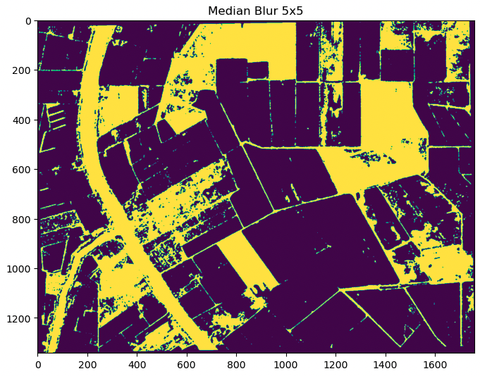
Create a segmentation masks from the classifier

The creation of a segmentation masks utilizing the predictions from the KNN classifier on the check dataset entails cleansing up the anticipated output to keep away from small segments attributable to picture noise. To take away speckle noise, we use the OpenCV median blur filter. This filter preserves street delineations between crops higher than the morphological open operation.

To use binary segmentation to the denoised output, we first have to convert the categorised raster knowledge to vector options utilizing the OpenCV findContours operate.

Lastly, the precise segmented crop areas may be computed utilizing the segmented crop outlines.

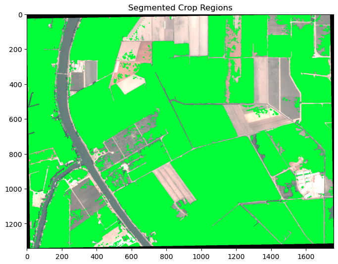
The segmented crop areas produced from the KNN classifier enable for exact identification of crop areas within the check dataset. These segmented areas can be utilized for numerous functions, similar to area boundary identification, crop monitoring, yield estimation, and useful resource allocation. The achieved F1 rating of 0.77 is nice and offers proof that the KNN classifier is an efficient instrument for crop segmentation in distant sensing photos. These outcomes can be utilized to additional enhance and refine crop segmentation strategies, doubtlessly resulting in elevated accuracy and effectivity in crop evaluation.

Conclusion

This submit demonstrated how you need to use the mixture of Planet’s excessive cadence, high-resolution satellite tv for pc imagery and SageMaker geospatial capabilities to carry out crop segmentation evaluation, unlocking precious insights that may enhance agricultural effectivity, environmental sustainability, and meals safety. Precisely figuring out crop areas permits additional evaluation on crop progress and productiveness, monitoring of land use modifications, and detection of potential meals safety dangers.

Furthermore, the mixture of Planet knowledge and SageMaker presents a variety of use instances past crop segmentation. The insights can allow data-driven choices on crop administration, useful resource allocation, and coverage planning in agriculture alone. With totally different knowledge and ML fashions, the mixed providing might additionally develop into different industries and use instances in the direction of digital transformation, sustainability transformation, and safety.

To start out utilizing SageMaker geospatial capabilities, see Get started with Amazon SageMaker geospatial capabilities.

To study extra about Planet’s imagery specs and developer reference supplies, go to Planet Developer’s Center. For documentation on Planet’s SDK for Python, see Planet SDK for Python. For extra details about Planet, together with its present knowledge merchandise and upcoming product releases, go to https://www.planet.com/.

Planet Labs PBC Ahead-Wanting Statements

Aside from the historic data contained herein, the issues set forth on this weblog submit are forward-looking statements inside the that means of the “secure harbor” provisions of the Personal Securities Litigation Reform Act of 1995, together with, however not restricted to, Planet Labs PBC’s potential to seize market alternative and notice any of the potential advantages from present or future product enhancements, new merchandise, or strategic partnerships and buyer collaborations. Ahead-looking statements are primarily based on Planet Labs PBC’s administration’s beliefs, in addition to assumptions made by, and knowledge at the moment accessible to them. As a result of such statements are primarily based on expectations as to future occasions and outcomes and are usually not statements of truth, precise outcomes might differ materially from these projected. Elements which can trigger precise outcomes to vary materially from present expectations embrace, however are usually not restricted to the danger elements and different disclosures about Planet Labs PBC and its enterprise included in Planet Labs PBC’s periodic experiences, proxy statements, and different disclosure supplies filed infrequently with the Securities and Trade Fee (SEC) which can be found on-line at www.sec.gov, and on Planet Labs PBC’s web site at www.planet.com. All forward-looking statements replicate Planet Labs PBC’s beliefs and assumptions solely as of the date such statements are made. Planet Labs PBC undertakes no obligation to replace forward-looking statements to replicate future occasions or circumstances.

Concerning the authors

Lydia Lihui Zhang is the Enterprise Growth Specialist at Planet Labs PBC, the place she helps join area for the betterment of earth throughout numerous sectors and a myriad of use instances. Beforehand, she was a knowledge scientist at McKinsey ACRE, an agriculture-focused answer. She holds a Grasp of Science from MIT Know-how Coverage Program, specializing in area coverage. Geospatial knowledge and its broader impression on enterprise and sustainability have been her profession focus.

Mansi Shah is a software program engineer, knowledge scientist, and musician whose work explores the areas the place inventive rigor and technical curiosity collide. She believes knowledge (like artwork!) imitates life, and is within the profoundly human tales behind the numbers and notes.

Xiong Zhou is a Senior Utilized Scientist at AWS. He leads the science group for Amazon SageMaker geospatial capabilities. His present space of analysis consists of pc imaginative and prescient and environment friendly mannequin coaching. In his spare time, he enjoys working, taking part in basketball, and spending time along with his household.

Janosch Woschitz is a Senior Options Architect at AWS, specializing in geospatial AI/ML. With over 15 years of expertise, he helps clients globally in leveraging AI and ML for revolutionary options that capitalize on geospatial knowledge. His experience spans machine studying, knowledge engineering, and scalable distributed programs, augmented by a powerful background in software program engineering and trade experience in complicated domains similar to autonomous driving.

Shital Dhakal is a Sr. Program Supervisor with the SageMaker geospatial ML group primarily based within the San Francisco Bay Space. He has a background in distant sensing and Geographic Info System (GIS). He’s obsessed with understanding clients ache factors and constructing geospatial merchandise to resolve them. In his spare time, he enjoys mountain climbing, touring, and taking part in tennis.