Past Numpy and Pandas: Unlocking the Potential of Lesser-Identified Python Libraries

Picture by OrMaVaredo on Pixabay

Python is among the most used programming languages on this planet and offers builders with a variety of libraries.

Anyway, with regards to information manipulation and scientific computation, we usually consider libraries similar to Numpy, Pandas, or SciPy.

On this article, we introduce 3 Python libraries chances are you’ll be eager about.

Introducing Dask

Dask is a versatile parallel computing library that permits distributed computing and parallelism for large-scale information processing.

So, why ought to we use Dask? As they are saying on their website:

Python has grown to change into the dominant language each in information analytics and basic programming. This development has been fueled by computational libraries like NumPy, pandas, and scikit-learn. Nevertheless, these packages weren’t designed to scale past a single machine. Dask was developed to natively scale these packages and the encircling ecosystem to multi-core machines and distributed clusters when datasets exceed reminiscence.

So, one of many frequent makes use of of Dask, as they say, is:

Dask DataFrame is utilized in conditions the place pandas is usually wanted, normally when pandas fails resulting from information dimension or computation velocity:
– Manipulating giant datasets, even when these datasets don’t slot in reminiscence
– Accelerating lengthy computations through the use of many cores
– Distributed computing on giant datasets with customary pandas operations like groupby, be a part of, and time collection computations

So, Dask is an efficient selection when we have to take care of large Pandas information frames. It is because Dask:

Permits customers to govern 100GB+ datasets on a laptop computer or 1TB+ datasets on a workstation

Which is a fairly spectacular outcome.

What occurs underneath the hood, is that:

Dask DataFrames coordinate many pandas DataFrames/Collection organized alongside the index. A Dask DataFrame is partitioned row-wise, grouping rows by index worth for effectivity. These pandas objects could dwell on disk or on different machines.

So, we’ve got one thing like that:

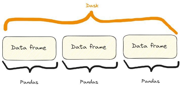
The distinction between a Dask and a Pandas information body. Picture by Creator, freely impressed by one on the Dask web site already quoted.

Some options of Dask in motion

To begin with, we have to set up Dask. We will do it through pip or conda like so:

$ pip set up dask[complete]

or

$ conda set up dask

FEATURE ONE: OPENING A CSV FILE

The primary function we will present of Dask is how we will open a CSV. We will do it like so:

import dask.dataframe as dd

# Load a big CSV file utilizing Dask
df_dask = dd.read_csv('my_very_large_dataset.csv')

# Carry out operations on the Dask DataFrame
mean_value_dask = df_dask['column_name'].imply().compute()

So, as we will see within the code, the best way we use Dask is similar to Pandas. Specifically:

• We use the strategy read_csv() precisely as in Pandas
• We intercept a column precisely as in Pandas. In reality, if we had a Pandas information body referred to as df we’d intercept a column this fashion: df['column_name'].
• We apply the imply() technique to the intercepted column much like Pandas, however right here we additionally want so as to add the strategy compute().

Additionally, even when the methodology of opening a CSV file it’s the identical as in Pandas, underneath the hood Dask is effortlessly processing a big dataset that exceeds the reminiscence capability of a single machine.

Because of this we will’t see any precise distinction, besides the truth that a big information body can’t be opened in Pandas, however in Dask we will.

FEATURE TWO: SCALING MACHINE LEARNING WORKFLOWS

We will use Dask to additionally create a classification dataset with an enormous variety of samples. We will then cut up it into the prepare and the check units, match the prepare set with an ML mannequin, and calculate predictions for the check set.

We will do it like so:

import dask_ml.datasets as dask_datasets
from dask_ml.linear_model import LogisticRegression
from dask_ml.model_selection import train_test_split

# Load a classification dataset utilizing Dask
X, y = dask_datasets.make_classification(n_samples=100000, chunks=1000)

# Break up the information into prepare and check units
X_train, X_test, y_train, y_test = train_test_split(X, y)

# Practice a logistic regression mannequin in parallel
mannequin = LogisticRegression()
mannequin.match(X_train, y_train)

# Predict on the check set
y_pred = mannequin.predict(X_test).compute()

This instance stresses the flexibility of Dask to deal with large datasets even within the case of a Machine Studying drawback, by distributing computations throughout a number of cores.

Specifically, we will create a “Dask dataset” for a classification case with the strategy dask_datasets.make_classification(), and we will specify the variety of samples and chunks (even, very large!).

Equally as earlier than, the predictions are obtained with the strategy compute().

NOTE:

on this case, chances are you'll have to intsall the module dask_ml.

You are able to do it like so:

$ pip set up dask_ml

FEATURE THREE: EFFICIENT IMAGE PROCESSING

The ability of parallel processing that Dask makes use of may also be utilized to photographs.

Specifically, we may open a number of photographs, resize them, and save them resized. We will do it like so:

import dask.array as da
import dask_image.imread
from PIL import Picture

# Load a set of photographs utilizing Dask
photographs = dask_image.imread.imread('picture*.jpg')

# Resize the photographs in parallel
resized_images = da.stack([da.resize(image, (300, 300)) for image in images])

# Compute the outcome
outcome = resized_images.compute()

# Save the resized photographs
for i, picture in enumerate(outcome):
    resized_image = Picture.fromarray(picture)
    resized_image.save(f'resized_image_{i}.jpg')

So, right here’s the method:

1. We open all of the “.jpg” photographs within the present folder (or in a folder you can specify) with the strategy dask_image.imread.imread("picture*.jpg").
2. We resize all of them at 300×300 utilizing a listing comprehension within the technique da.stack().
3. We compute the outcome with the strategy compute(), as we did earlier than.
4. We save all of the resized photographs with the for cycle.

Introducing Sympy

If you’ll want to make mathematical calculations and computations and wish to follow Python, you’ll be able to strive Sympy.

Certainly: why use different instruments and software program, once we can use our beloved Python?

As per what they write on their website, Sympy is:

A Python library for symbolic arithmetic. It goals to change into a full-featured pc algebra system (CAS) whereas protecting the code so simple as attainable with a purpose to be understandable and simply extensible. SymPy is written totally in Python.

However why use SymPy? They counsel:

SymPy is…

– Free: Licensed underneath BSD, SymPy is free each as in speech and as in beer.

– Python-based: SymPy is written totally in Python and makes use of Python for its language.

– Light-weight: SymPy solely is determined by mpmath, a pure Python library for arbitrary floating level arithmetic, making it simple to make use of.

– A library: Past use as an interactive software, SymPy could be embedded in different purposes and prolonged with customized capabilities.

So, it mainly has all of the traits that may be liked by Python addicts!

Now, let’s see a few of its options.

Some options of SymPy in motion

To begin with, we have to set up it:

PAY ATTENTION:

should you write $ pip set up simpy you will set up one other (fully

completely different!) library.

So, the second letter is a "y", not an "i".

FEATURE ONE: SOLVING AN ALGEBRAIC EQUATION

If we have to resolve an algebraic equation, we will use SymPy like so:

from sympy import symbols, Eq, resolve

# Outline the symbols
x, y = symbols('x y')

# Outline the equation
equation = Eq(x**2 + y**2, 25)

# Clear up the equation
options = resolve(equation, (x, y))

# Print answer
print(options)


>>>


[(-sqrt(25 - y**2), y), (sqrt(25 - y**2), y)]

So, that’s the method:

1. We outline the symbols of the equation with the strategy symbols().
2. We write the algebraic equation with the strategy Eq.
3. We resolve the equation with the strategy resolve().

After I was on the College I used completely different instruments to resolve these sorts of issues, and I’ve to say that SymPy, as we will see, could be very readable and user-friendly.

However, certainly: it’s a Python library, so how may that be any completely different?

FEATURE TWO: CALCULATING DERIVATIVES

Calculating derivatives is one other job we could mathematically want, for lots of causes when analyzing information. Usually, we may have calculations for any motive, and SympY actually simplifies this course of. In reality, we will do it like so:

from sympy import symbols, diff

# Outline the image
x = symbols('x')

# Outline the operate
f = x**3 + 2*x**2 + 3*x + 4

# Calculate the by-product
by-product = diff(f, x)

# Print by-product
print(by-product)

>>>

3*x**2 + 4*x + 3

So, as we will see, the method could be very easy and self-explainable:

1. We outline the image of the operate we’re deriving with symbols().
2. We outline the operate.
3. We calculate the by-product with diff() specifying the operate and the image we’re calculating the by-product (that is an absolute by-product, however we may carry out even partial derivatives within the case of capabilities which have x and y variables).

And if we check it, we’ll see that the outcome arrives in a matter of two or 3 seconds. So, it’s additionally fairly quick.

FEATURE THREE: CALCULATING INTEGRATIONS

In fact, if SymPy can calculate derivatives, it could additionally calculate integrations. Let’s do it:

from sympy import symbols, combine, sin

# Outline the image
x = symbols('x')

# Carry out symbolic integration
integral = combine(sin(x), x)

# Print integral
print(integral)

>>>

-cos(x)

So, right here we use the strategy combine(), specifying the operate to combine and the variable of integration.

Couldn’t it’s simpler?!

Introducing Xarray

Xarray is a Python library that extends the options and functionalities of NumPy, giving us the chance to work with labeled arrays and datasets.

As they are saying on their website, in truth:

Xarray makes working with labeled multi-dimensional arrays in Python easy, environment friendly, and enjoyable!

And also:

Xarray introduces labels within the type of dimensions, coordinates and attributes on high of uncooked NumPy-like multidimensional arrays, which permits for a extra intuitive, extra concise, and fewer error-prone developer expertise.

In different phrases, it extends the performance of NumPy arrays by including labels or coordinates to the array dimensions. These labels present metadata and allow extra superior evaluation and manipulation of multi-dimensional information.

For instance, in NumPy, arrays are accessed utilizing integer-based indexing.

In Xarray, as a substitute, every dimension can have a label related to it, making it simpler to grasp and manipulate the information primarily based on significant names.

For instance, as a substitute of accessing information with arr[0, 1, 2], we will use arr.sel(x=0, y=1, z=2) in Xarray, the place x, y, and z are dimension labels.

This makes the code far more readable!

So, let’s see some options of Xarray.

Some options of Xarray in motion

As common, to put in it:

FEATURE ONE: WORKING WITH LABELED COORDINATES

Suppose we wish to create some information associated to temperature and we wish to label these with coordinates like latitude and longitude. We will do it like so:

import xarray as xr
import numpy as np

# Create temperature information
temperature = np.random.rand(100, 100) * 20 + 10

# Create coordinate arrays for latitude and longitude
latitudes = np.linspace(-90, 90, 100)
longitudes = np.linspace(-180, 180, 100)

# Create an Xarray information array with labeled coordinates
da = xr.DataArray(
    temperature,
    dims=['latitude', 'longitude'],
    coords={'latitude': latitudes, 'longitude': longitudes}
)

# Entry information utilizing labeled coordinates
subset = da.sel(latitude=slice(-45, 45), longitude=slice(-90, 0))

And if we print them we get:

# Print information
print(subset)

>>>

array([[13.45064786, 29.15218061, 14.77363206, ..., 12.00262833,
        16.42712411, 15.61353963],
       [23.47498117, 20.25554247, 14.44056286, ..., 19.04096482,
        15.60398491, 24.69535367],
       [25.48971105, 20.64944534, 21.2263141 , ..., 25.80933737,
        16.72629302, 29.48307134],
       ...,
       [10.19615833, 17.106716  , 10.79594252, ..., 29.6897709 ,
        20.68549602, 29.4015482 ],
       [26.54253304, 14.21939699, 11.085207  , ..., 15.56702191,
        19.64285595, 18.03809074],
       [26.50676351, 15.21217526, 23.63645069, ..., 17.22512125,
        13.96942377, 13.93766583]])
Coordinates:
  * latitude   (latitude) float64 -44.55 -42.73 -40.91 ... 40.91 42.73 44.55
  * longitude  (longitude) float64 -89.09 -85.45 -81.82 ... -9.091 -5.455 -1.818

So, let’s see the method step-by-step:

1. We’ve created the temperature values as a NumPy array.
2. We’ve outlined the latitudes and longitueas values as NumPy arrays.
3. We’ve saved all the information in an Xarray array with the strategy DataArray().
4. We’ve chosen a subset of the latitudes and longitudes with the strategy sel() that selects the values we would like for our subset.

The outcome can be simply readable, so labeling is admittedly useful in numerous circumstances.

FEATURE TWO: HANDLING MISSING DATA

Suppose we’re amassing information associated to temperatures in the course of the yr. We wish to know if we’ve got some null values in our array. Here is how we will accomplish that:

import xarray as xr
import numpy as np
import pandas as pd

# Create temperature information with lacking values
temperature = np.random.rand(365, 50, 50) * 20 + 10
temperature[0:10, :, :] = np.nan  # Set the primary 10 days as lacking values

# Create time, latitude, and longitude coordinate arrays
instances = pd.date_range('2023-01-01', durations=365, freq='D')
latitudes = np.linspace(-90, 90, 50)
longitudes = np.linspace(-180, 180, 50)

# Create an Xarray information array with lacking values
da = xr.DataArray(
    temperature,
    dims=['time', 'latitude', 'longitude'],
    coords={'time': instances, 'latitude': latitudes, 'longitude': longitudes}
)

# Rely the variety of lacking values alongside the time dimension
missing_count = da.isnull().sum(dim='time')

# Print lacking values
print(missing_count)

>>>


array([[10, 10, 10, ..., 10, 10, 10],
       [10, 10, 10, ..., 10, 10, 10],
       [10, 10, 10, ..., 10, 10, 10],
       ...,
       [10, 10, 10, ..., 10, 10, 10],
       [10, 10, 10, ..., 10, 10, 10],
       [10, 10, 10, ..., 10, 10, 10]])
Coordinates:
  * latitude   (latitude) float64 -90.0 -86.33 -82.65 ... 82.65 86.33 90.0
  * longitude  (longitude) float64 -180.0 -172.7 -165.3 ... 165.3 172.7 180.0

And so we get hold of that we’ve got 10 null values.

Additionally, if we have a look carefully on the code, we will see that we will apply Pandas’ strategies to an Xarray like isnull.sum(), as on this case, that counts the whole variety of lacking values.

FEATURE ONE: HANDLING AND ANALYZING MULTI-DIMENSIONAL DATA

The temptation to deal with and analyze multi-dimensional information is excessive when we’ve got the chance to label our arrays. So, why not strive it?

For instance, suppose we’re nonetheless amassing information associated to temperatures at sure latitudes and longitudes.

We could wish to calculate the imply, the max, and the median temperatures. We will do it like so:

import xarray as xr
import numpy as np
import pandas as pd

# Create artificial temperature information
temperature = np.random.rand(365, 50, 50) * 20 + 10

# Create time, latitude, and longitude coordinate arrays
instances = pd.date_range('2023-01-01', durations=365, freq='D')
latitudes = np.linspace(-90, 90, 50)
longitudes = np.linspace(-180, 180, 50)

# Create an Xarray dataset
ds = xr.Dataset(
    {
        'temperature': (['time', 'latitude', 'longitude'], temperature),
    },
    coords={
        'time': instances,
        'latitude': latitudes,
        'longitude': longitudes,
    }
)

# Carry out statistical evaluation on the temperature information
mean_temperature = ds['temperature'].imply(dim='time')
max_temperature = ds['temperature'].max(dim='time')
min_temperature = ds['temperature'].min(dim='time')

# Print values 
print(f"imply temperature:n {mean_temperature}n")
print(f"max temperature:n {max_temperature}n")
print(f"min temperature:n {min_temperature}n")


>>>

imply temperature:
 
array([[19.99931701, 20.36395016, 20.04110699, ..., 19.98811842,
        20.08895803, 19.86064693],
       [19.84016491, 19.87077812, 20.27445405, ..., 19.8071972 ,
        19.62665953, 19.58231185],
       [19.63911165, 19.62051976, 19.61247548, ..., 19.85043831,
        20.13086891, 19.80267099],
       ...,
       [20.18590514, 20.05931149, 20.17133483, ..., 20.52858247,
        19.83882433, 20.66808513],
       [19.56455575, 19.90091128, 20.32566232, ..., 19.88689221,
        19.78811145, 19.91205212],
       [19.82268297, 20.14242279, 19.60842148, ..., 19.68290006,
        20.00327294, 19.68955107]])
Coordinates:
  * latitude   (latitude) float64 -90.0 -86.33 -82.65 ... 82.65 86.33 90.0
  * longitude  (longitude) float64 -180.0 -172.7 -165.3 ... 165.3 172.7 180.0

max temperature:
 
array([[29.98465531, 29.97609171, 29.96821276, ..., 29.86639343,
        29.95069558, 29.98807808],
       [29.91802049, 29.92870312, 29.87625447, ..., 29.92519055,
        29.9964299 , 29.99792388],
       [29.96647016, 29.7934891 , 29.89731136, ..., 29.99174546,
        29.97267052, 29.96058079],
       ...,
       [29.91699117, 29.98920555, 29.83798369, ..., 29.90271746,
        29.93747041, 29.97244906],
       [29.99171911, 29.99051943, 29.92706773, ..., 29.90578739,
        29.99433847, 29.94506567],
       [29.99438621, 29.98798699, 29.97664488, ..., 29.98669576,
        29.91296382, 29.93100249]])
Coordinates:
  * latitude   (latitude) float64 -90.0 -86.33 -82.65 ... 82.65 86.33 90.0
  * longitude  (longitude) float64 -180.0 -172.7 -165.3 ... 165.3 172.7 180.0

min temperature:
 
array([[10.0326431 , 10.07666029, 10.02795524, ..., 10.17215336,
        10.00264909, 10.05387097],
       [10.00355858, 10.00610942, 10.02567816, ..., 10.29100316,
        10.00861792, 10.16955806],
       [10.01636216, 10.02856619, 10.00389027, ..., 10.0929342 ,
        10.01504103, 10.06219179],
       ...,
       [10.00477003, 10.0303088 , 10.04494723, ..., 10.05720692,
        10.122994  , 10.04947012],
       [10.00422182, 10.0211205 , 10.00183528, ..., 10.03818058,
        10.02632697, 10.06722953],
       [10.10994581, 10.12445222, 10.03002468, ..., 10.06937041,
        10.04924046, 10.00645499]])
Coordinates:
  * latitude   (latitude) float64 -90.0 -86.33 -82.65 ... 82.65 86.33 90.0
  * longitude  (longitude) float64 -180.0 -172.7 -165.3 ... 165.3 172.7 180.0

And we obtained what we wished, additionally in a clearly readable manner.

And once more, as earlier than, to calculate the max, min, and imply values of temperatures we’ve used Pandas’ capabilities utilized to an array.

On this article, we’ve proven three libraries for scientific calculation and computation.

Whereas SymPy could be the substitute for different instruments and software program, giving us the chance to make use of Python code to compute mathematical calculations, Dask and Xarray lengthen the functionalities of different libraries, serving to us in conditions the place we could have difficulties with different most recognized Python libraries for information evaluation and manipulation.

 
 
Federico Trotta has liked writing since he was a younger boy in class, writing detective tales as class exams. Due to his curiosity, he found programming and AI. Having a burning ardour for writing, he could not keep away from beginning to write about these matters, so he determined to vary his profession to change into a Technical Author. His objective is to coach folks on Python programming, Machine Studying, and Knowledge Science, by means of writing. Discover extra about him at federicotrotta.com.

 
Original. Reposted with permission.