Instruments for TensorFlow Coaching Runs

The tfruns package supplies a collection of instruments for monitoring, visualizing, and managing TensorFlow coaching runs and experiments from R. Use the tfruns package deal to:

• Monitor the hyperparameters, metrics, output, and supply code of each coaching run.

• Evaluate hyperparmaeters and metrics throughout runs to search out the most effective performing mannequin.

• Routinely generate studies to visualise particular person coaching runs or comparisons between runs.
  

You’ll be able to set up the tfruns package deal from GitHub as follows:

devtools::install_github("rstudio/tfruns")

Full documentation for tfruns is obtainable on the TensorFlow for R website.

tfruns is meant for use with the keras and/or the tfestimators packages, each of which give greater stage interfaces to TensorFlow from R. These packages might be put in with:

# keras
install.packages("keras")

# tfestimators
devtools::install_github("rstudio/tfestimators")

Coaching

Within the following sections we’ll describe the varied capabilities of tfruns. Our instance coaching script (mnist_mlp.R) trains a Keras mannequin to acknowledge MNIST digits.

To coach a mannequin with tfruns, simply use the training_run() operate rather than the supply() operate to execute your R script. For instance:

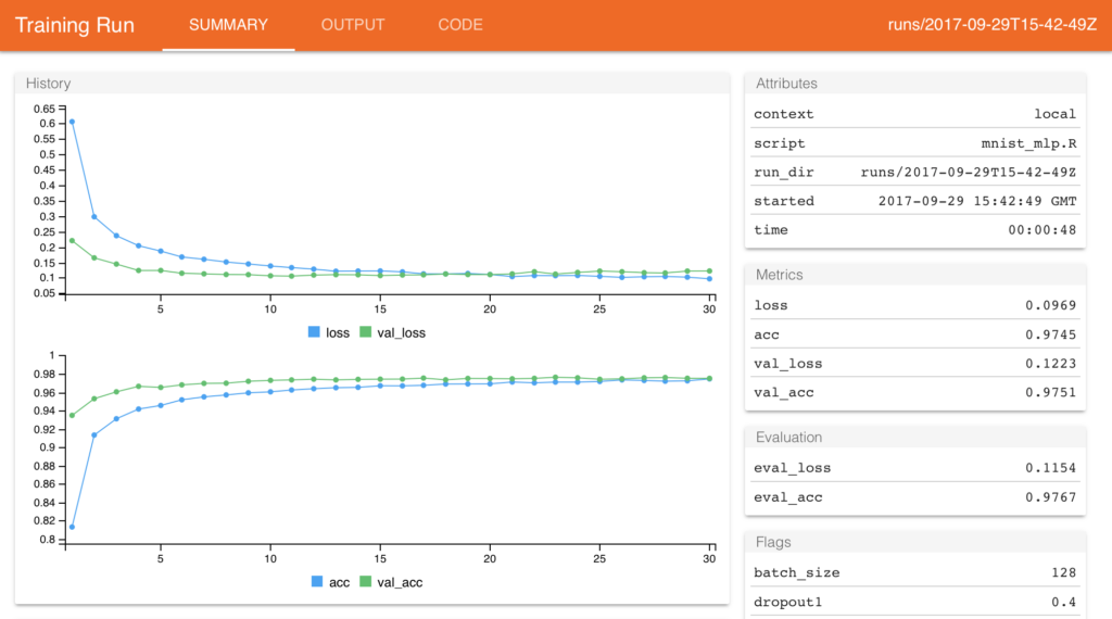
When coaching is accomplished, a abstract of the run will routinely be displayed if you’re inside an interactive R session:

The metrics and output of every run are routinely captured inside a run listing which is exclusive for every run that you just provoke. Observe that for Keras and TF Estimator fashions this knowledge is captured routinely (no adjustments to your supply code are required).

You’ll be able to name the latest_run() operate to view the outcomes of the final run (together with the trail to the run listing which shops all the run’s output):

$ run_dir           : chr "runs/2017-10-02T14-23-38Z"
$ eval_loss         : num 0.0956
$ eval_acc          : num 0.98
$ metric_loss       : num 0.0624
$ metric_acc        : num 0.984
$ metric_val_loss   : num 0.0962
$ metric_val_acc    : num 0.98
$ flag_dropout1     : num 0.4
$ flag_dropout2     : num 0.3
$ samples           : int 48000
$ validation_samples: int 12000
$ batch_size        : int 128
$ epochs            : int 20
$ epochs_completed  : int 20
$ metrics           : chr "(metrics knowledge body)"
$ mannequin             : chr "(mannequin abstract)"
$ loss_function     : chr "categorical_crossentropy"
$ optimizer         : chr "RMSprop"
$ learning_rate     : num 0.001
$ script            : chr "mnist_mlp.R"
$ begin             : POSIXct[1:1], format: "2017-10-02 14:23:38"
$ finish               : POSIXct[1:1], format: "2017-10-02 14:24:24"
$ accomplished         : logi TRUE
$ output            : chr "(script ouptut)"
$ source_code       : chr "(supply archive)"
$ context           : chr "native"
$ sort              : chr "coaching"

The run listing used within the instance above is “runs/2017-10-02T14-23-38Z”. Run directories are by default generated inside the “runs” subdirectory of the present working listing, and use a timestamp because the title of the run listing. You’ll be able to view the report for any given run utilizing the view_run() operate:

view_run("runs/2017-10-02T14-23-38Z")

Evaluating Runs

Let’s make a few adjustments to our coaching script to see if we are able to enhance mannequin efficiency. We’ll change the variety of items in our first dense layer to 128, change the learning_rate from 0.001 to 0.003 and run 30 relatively than 20 epochs. After making these adjustments to the supply code we re-run the script utilizing training_run() as earlier than:

training_run("mnist_mlp.R")

This may even present us a report summarizing the outcomes of the run, however what we’re actually all in favour of is a comparability between this run and the earlier one. We will view a comparability by way of the compare_runs() operate:

The comparability report reveals the mannequin attributes and metrics side-by-side, in addition to variations within the supply code and output of the coaching script.

Observe that compare_runs() will by default examine the final two runs, nevertheless you may cross any two run directories you wish to be in contrast.

Utilizing Flags

Tuning a mannequin typically requires exploring the impression of adjustments to many hyperparameters. One of the best ways to method that is typically not by altering the supply code of the coaching script as we did above, however as a substitute by defining flags for key parameters it’s possible you’ll wish to fluctuate. Within the instance script you may see that now we have accomplished this for the dropout layers:

FLAGS <- flags(
  flag_numeric("dropout1", 0.4),
  flag_numeric("dropout2", 0.3)
)

These flags are then used within the definition of our mannequin right here:

mannequin <- keras_model_sequential()
mannequin %>%
  layer_dense(items = 128, activation = 'relu', input_shape = c(784)) %>%
  layer_dropout(charge = FLAGS$dropout1) %>%
  layer_dense(items = 128, activation = 'relu') %>%
  layer_dropout(charge = FLAGS$dropout2) %>%
  layer_dense(items = 10, activation = 'softmax')

As soon as we’ve outlined flags, we are able to cross alternate flag values to training_run() as follows:

training_run('mnist_mlp.R', flags = c(dropout1 = 0.2, dropout2 = 0.2))

You aren’t required to specify all the flags (any flags excluded will merely use their default worth).

Flags make it very easy to systematically discover the impression of adjustments to hyperparameters on mannequin efficiency, for instance:

for (dropout1 in c(0.1, 0.2, 0.3))
  training_run('mnist_mlp.R', flags = c(dropout1 = dropout1))

Flag values are routinely included in run knowledge with a “flag_” prefix (e.g. flag_dropout1, flag_dropout2).

See the article on training flags for extra documentation on utilizing flags.

Analyzing Runs

We’ve demonstrated visualizing and evaluating one or two runs, nevertheless as you accumulate extra runs you’ll typically wish to analyze and examine runs many runs. You should use the ls_runs() operate to yield a knowledge body with abstract info on all the runs you’ve performed inside a given listing:

# A tibble: 6 x 27
                    run_dir eval_loss eval_acc metric_loss metric_acc metric_val_loss
                      <chr>     <dbl>    <dbl>       <dbl>      <dbl>           <dbl>
1 runs/2017-10-02T14-56-57Z    0.1263   0.9784      0.0773     0.9807          0.1283
2 runs/2017-10-02T14-56-04Z    0.1323   0.9783      0.0545     0.9860          0.1414
3 runs/2017-10-02T14-55-11Z    0.1407   0.9804      0.0348     0.9914          0.1542
4 runs/2017-10-02T14-51-44Z    0.1164   0.9801      0.0448     0.9882          0.1396
5 runs/2017-10-02T14-37-00Z    0.1338   0.9750      0.1097     0.9732          0.1328
6 runs/2017-10-02T14-23-38Z    0.0956   0.9796      0.0624     0.9835          0.0962
# ... with 21 extra variables: metric_val_acc <dbl>, flag_dropout1 <dbl>,
#   flag_dropout2 <dbl>, samples <int>, validation_samples <int>, batch_size <int>,
#   epochs <int>, epochs_completed <int>, metrics <chr>, mannequin <chr>, loss_function <chr>,
#   optimizer <chr>, learning_rate <dbl>, script <chr>, begin <dttm>, finish <dttm>,
#   accomplished <lgl>, output <chr>, source_code <chr>, context <chr>, sort <chr>

Since ls_runs() returns a knowledge body it’s also possible to render a sortable, filterable model of it inside RStudio utilizing the View() operate:

The ls_runs() operate additionally helps subset and order arguments. For instance, the next will yield all runs with an eval accuracy higher than 0.98:

ls_runs(eval_acc > 0.98, order = eval_acc)

You’ll be able to cross the outcomes of ls_runs() to match runs (which is able to at all times examine the primary two runs handed). For instance, it will examine the 2 runs that carried out finest when it comes to analysis accuracy:

compare_runs(ls_runs(eval_acc > 0.98, order = eval_acc))

RStudio IDE

When you use RStudio with tfruns, it’s strongly advisable that you just replace to the present Preview Release of RStudio v1.1, as there are are quite a few factors of integration with the IDE that require this newer launch.

Addin

The tfruns package deal installs an RStudio IDE addin which supplies fast entry to often used capabilities from the Addins menu:

Observe that you need to use Instruments -> Modify Keyboard Shortcuts inside RStudio to assign a keyboard shortcut to a number of of the addin instructions.

Background Coaching

RStudio v1.1 features a Terminal pane alongside the Console pane. Since coaching runs can develop into fairly prolonged, it’s typically helpful to run them within the background with a view to hold the R console free for different work. You are able to do this from a Terminal as follows:

If you’re not operating inside RStudio then you may in fact use a system terminal window for background coaching.

Publishing Studies

Coaching run views and comparisons are HTML paperwork which might be saved and shared with others. When viewing a report inside RStudio v1.1 it can save you a replica of the report or publish it to RPubs or RStudio Join:

If you’re not operating inside RStudio then you need to use the save_run_view() and save_run_comparison() capabilities to create standalone HTML variations of run studies.

Managing Runs

There are a number of instruments out there for managing coaching run output, together with:

1. Exporting run artifacts (e.g. saved fashions).

2. Copying and purging run directories.

3. Utilizing a customized run listing for an experiment or different set of associated runs.

The Managing Runs article supplies extra particulars on utilizing these options.