Picture Classification on Small Datasets with Keras

Coaching a convnet with a small dataset

Having to coach an image-classification mannequin utilizing little or no knowledge is a standard scenario, which you’ll possible encounter in observe if you happen to ever do laptop imaginative and prescient in an expert context. A “few” samples can imply anyplace from just a few hundred to a couple tens of 1000’s of photos. As a sensible instance, we’ll deal with classifying photos as canines or cats, in a dataset containing 4,000 footage of cats and canines (2,000 cats, 2,000 canines). We’ll use 2,000 footage for coaching – 1,000 for validation, and 1,000 for testing.

In Chapter 5 of the Deep Learning with R ebook we overview three strategies for tackling this drawback. The primary of those is coaching a small mannequin from scratch on what little knowledge you might have (which achieves an accuracy of 82%). Subsequently we use function extraction with a pretrained community (leading to an accuracy of 90%) and fine-tuning a pretrained community (with a ultimate accuracy of 97%). On this submit we’ll cowl solely the second and third strategies.

The relevance of deep studying for small-data issues

You’ll typically hear that deep studying solely works when numerous knowledge is out there. That is legitimate partly: one basic attribute of deep studying is that it may well discover fascinating options within the coaching knowledge by itself, with none want for handbook function engineering, and this could solely be achieved when numerous coaching examples can be found. That is very true for issues the place the enter samples are very high-dimensional, like photos.

However what constitutes numerous samples is relative – relative to the dimensions and depth of the community you’re making an attempt to coach, for starters. It isn’t attainable to coach a convnet to unravel a fancy drawback with only a few tens of samples, however just a few hundred can probably suffice if the mannequin is small and nicely regularized and the duty is straightforward. As a result of convnets study native, translation-invariant options, they’re extremely knowledge environment friendly on perceptual issues. Coaching a convnet from scratch on a really small picture dataset will nonetheless yield cheap outcomes regardless of a relative lack of information, with out the necessity for any customized function engineering. You’ll see this in motion on this part.

What’s extra, deep-learning fashions are by nature extremely repurposable: you possibly can take, say, an image-classification or speech-to-text mannequin educated on a large-scale dataset and reuse it on a considerably totally different drawback with solely minor modifications. Particularly, within the case of laptop imaginative and prescient, many pretrained fashions (normally educated on the ImageNet dataset) at the moment are publicly obtainable for obtain and can be utilized to bootstrap highly effective imaginative and prescient fashions out of little or no knowledge. That’s what you’ll do within the subsequent part. Let’s begin by getting your fingers on the info.

Downloading the info

The Canines vs. Cats dataset that you simply’ll use isn’t packaged with Keras. It was made obtainable by Kaggle as a part of a computer-vision competitors in late 2013, again when convnets weren’t mainstream. You may obtain the unique dataset from https://www.kaggle.com/c/dogs-vs-cats/data (you’ll have to create a Kaggle account if you happen to don’t have already got one – don’t fear, the method is painless).

The images are medium-resolution colour JPEGs. Listed here are some examples:

Unsurprisingly, the dogs-versus-cats Kaggle competitors in 2013 was gained by entrants who used convnets. The very best entries achieved as much as 95% accuracy. Under you’ll find yourself with a 97% accuracy, despite the fact that you’ll practice your fashions on lower than 10% of the info that was obtainable to the rivals.

This dataset comprises 25,000 photos of canines and cats (12,500 from every class) and is 543 MB (compressed). After downloading and uncompressing it, you’ll create a brand new dataset containing three subsets: a coaching set with 1,000 samples of every class, a validation set with 500 samples of every class, and a check set with 500 samples of every class.

Following is the code to do that:

original_dataset_dir <- "~/Downloads/kaggle_original_data"

base_dir <- "~/Downloads/cats_and_dogs_small"
dir.create(base_dir)

train_dir <- file.path(base_dir, "practice")
dir.create(train_dir)
validation_dir <- file.path(base_dir, "validation")
dir.create(validation_dir)
test_dir <- file.path(base_dir, "check")
dir.create(test_dir)

train_cats_dir <- file.path(train_dir, "cats")
dir.create(train_cats_dir)

train_dogs_dir <- file.path(train_dir, "canines")
dir.create(train_dogs_dir)

validation_cats_dir <- file.path(validation_dir, "cats")
dir.create(validation_cats_dir)

validation_dogs_dir <- file.path(validation_dir, "canines")
dir.create(validation_dogs_dir)

test_cats_dir <- file.path(test_dir, "cats")
dir.create(test_cats_dir)

test_dogs_dir <- file.path(test_dir, "canines")
dir.create(test_dogs_dir)

fnames <- paste0("cat.", 1:1000, ".jpg")
file.copy(file.path(original_dataset_dir, fnames), 
          file.path(train_cats_dir)) 

fnames <- paste0("cat.", 1001:1500, ".jpg")
file.copy(file.path(original_dataset_dir, fnames), 
          file.path(validation_cats_dir))

fnames <- paste0("cat.", 1501:2000, ".jpg")
file.copy(file.path(original_dataset_dir, fnames),
          file.path(test_cats_dir))

fnames <- paste0("canine.", 1:1000, ".jpg")
file.copy(file.path(original_dataset_dir, fnames),
          file.path(train_dogs_dir))

fnames <- paste0("canine.", 1001:1500, ".jpg")
file.copy(file.path(original_dataset_dir, fnames),
          file.path(validation_dogs_dir)) 

fnames <- paste0("canine.", 1501:2000, ".jpg")
file.copy(file.path(original_dataset_dir, fnames),
          file.path(test_dogs_dir))

Utilizing a pretrained convnet

A typical and extremely efficient method to deep studying on small picture datasets is to make use of a pretrained community. A pretrained community is a saved community that was beforehand educated on a big dataset, usually on a large-scale image-classification activity. If this authentic dataset is massive sufficient and normal sufficient, then the spatial hierarchy of options discovered by the pretrained community can successfully act as a generic mannequin of the visible world, and therefore its options can show helpful for a lot of totally different computer-vision issues, despite the fact that these new issues could contain utterly totally different lessons than these of the unique activity. For example, you would possibly practice a community on ImageNet (the place lessons are largely animals and on a regular basis objects) after which repurpose this educated community for one thing as distant as figuring out furnishings objects in photos. Such portability of discovered options throughout totally different issues is a key benefit of deep studying in comparison with many older, shallow-learning approaches, and it makes deep studying very efficient for small-data issues.

On this case, let’s think about a big convnet educated on the ImageNet dataset (1.4 million labeled photos and 1,000 totally different lessons). ImageNet comprises many animal lessons, together with totally different species of cats and canines, and you may thus anticipate to carry out nicely on the dogs-versus-cats classification drawback.

You’ll use the VGG16 architecture, developed by Karen Simonyan and Andrew Zisserman in 2014; it’s a easy and extensively used convnet structure for ImageNet. Though it’s an older mannequin, removed from the present state-of-the-art and considerably heavier than many different latest fashions, I selected it as a result of its structure is much like what you’re already acquainted with and is straightforward to know with out introducing any new ideas. This can be your first encounter with one in all these cutesy mannequin names – VGG, ResNet, Inception, Inception-ResNet, Xception, and so forth; you’ll get used to them, as a result of they are going to come up regularly if you happen to preserve doing deep studying for laptop imaginative and prescient.

There are two methods to make use of a pretrained community: function extraction and fine-tuning. We’ll cowl each of them. Let’s begin with function extraction.

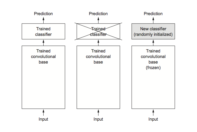
Characteristic extraction consists of utilizing the representations discovered by a earlier community to extract fascinating options from new samples. These options are then run by a brand new classifier, which is educated from scratch.

As you noticed beforehand, convnets used for picture classification comprise two elements: they begin with a sequence of pooling and convolution layers, they usually finish with a densely linked classifier. The primary half is known as the convolutional base of the mannequin. Within the case of convnets, function extraction consists of taking the convolutional base of a beforehand educated community, working the brand new knowledge by it, and coaching a brand new classifier on prime of the output.

Why solely reuse the convolutional base? May you reuse the densely linked classifier as nicely? Usually, doing so needs to be prevented. The reason being that the representations discovered by the convolutional base are more likely to be extra generic and due to this fact extra reusable: the function maps of a convnet are presence maps of generic ideas over an image, which is more likely to be helpful whatever the computer-vision drawback at hand. However the representations discovered by the classifier will essentially be particular to the set of lessons on which the mannequin was educated – they are going to solely comprise details about the presence chance of this or that class in your complete image. Moreover, representations present in densely linked layers now not comprise any details about the place objects are positioned within the enter picture: these layers do away with the notion of area, whereas the article location remains to be described by convolutional function maps. For issues the place object location issues, densely linked options are largely ineffective.

Observe that the extent of generality (and due to this fact reusability) of the representations extracted by particular convolution layers relies on the depth of the layer within the mannequin. Layers that come earlier within the mannequin extract native, extremely generic function maps (similar to visible edges, colours, and textures), whereas layers which can be increased up extract more-abstract ideas (similar to “cat ear” or “canine eye”). So in case your new dataset differs quite a bit from the dataset on which the unique mannequin was educated, you might be higher off utilizing solely the primary few layers of the mannequin to do function extraction, slightly than utilizing your complete convolutional base.

On this case, as a result of the ImageNet class set comprises a number of canine and cat lessons, it’s more likely to be helpful to reuse the data contained within the densely linked layers of the unique mannequin. However we’ll select to not, as a way to cowl the extra normal case the place the category set of the brand new drawback doesn’t overlap the category set of the unique mannequin.

Let’s put this in observe through the use of the convolutional base of the VGG16 community, educated on ImageNet, to extract fascinating options from cat and canine photos, after which practice a dogs-versus-cats classifier on prime of those options.

The VGG16 mannequin, amongst others, comes prepackaged with Keras. Right here’s the listing of image-classification fashions (all pretrained on the ImageNet dataset) which can be obtainable as a part of Keras:

• Xception
• Inception V3
• ResNet50
• VGG16
• VGG19
• MobileNet

Let’s instantiate the VGG16 mannequin.

library(keras)

conv_base <- application_vgg16(
  weights = "imagenet",
  include_top = FALSE,
  input_shape = c(150, 150, 3)
)

You move three arguments to the operate:

• weights specifies the burden checkpoint from which to initialize the mannequin.
• include_top refers to together with (or not) the densely linked classifier on prime of the community. By default, this densely linked classifier corresponds to the 1,000 lessons from ImageNet. Since you intend to make use of your personal densely linked classifier (with solely two lessons: cat and canine), you don’t want to incorporate it.
• input_shape is the form of the picture tensors that you simply’ll feed to the community. This argument is only optionally available: if you happen to don’t move it, the community will be capable of course of inputs of any dimension.

Right here’s the element of the structure of the VGG16 convolutional base. It’s much like the straightforward convnets you’re already acquainted with:

Layer (kind)                     Output Form          Param #  
================================================================
input_1 (InputLayer)             (None, 150, 150, 3)   0       
________________________________________________________________
block1_conv1 (Convolution2D)     (None, 150, 150, 64)  1792     
________________________________________________________________
block1_conv2 (Convolution2D)     (None, 150, 150, 64)  36928    
________________________________________________________________
block1_pool (MaxPooling2D)       (None, 75, 75, 64)    0        
________________________________________________________________
block2_conv1 (Convolution2D)     (None, 75, 75, 128)   73856    
________________________________________________________________
block2_conv2 (Convolution2D)     (None, 75, 75, 128)   147584   
________________________________________________________________
block2_pool (MaxPooling2D)       (None, 37, 37, 128)   0        
________________________________________________________________
block3_conv1 (Convolution2D)     (None, 37, 37, 256)   295168   
________________________________________________________________
block3_conv2 (Convolution2D)     (None, 37, 37, 256)   590080   
________________________________________________________________
block3_conv3 (Convolution2D)     (None, 37, 37, 256)   590080   
________________________________________________________________
block3_pool (MaxPooling2D)       (None, 18, 18, 256)   0        
________________________________________________________________
block4_conv1 (Convolution2D)     (None, 18, 18, 512)   1180160  
________________________________________________________________
block4_conv2 (Convolution2D)     (None, 18, 18, 512)   2359808  
________________________________________________________________
block4_conv3 (Convolution2D)     (None, 18, 18, 512)   2359808  
________________________________________________________________
block4_pool (MaxPooling2D)       (None, 9, 9, 512)     0        
________________________________________________________________
block5_conv1 (Convolution2D)     (None, 9, 9, 512)     2359808  
________________________________________________________________
block5_conv2 (Convolution2D)     (None, 9, 9, 512)     2359808  
________________________________________________________________
block5_conv3 (Convolution2D)     (None, 9, 9, 512)     2359808  
________________________________________________________________
block5_pool (MaxPooling2D)       (None, 4, 4, 512)     0        
================================================================
Whole params: 14,714,688
Trainable params: 14,714,688
Non-trainable params: 0

The ultimate function map has form (4, 4, 512). That’s the function on prime of which you’ll stick a densely linked classifier.

At this level, there are two methods you could possibly proceed:

• Operating the convolutional base over your dataset, recording its output to an array on disk, after which utilizing this knowledge as enter to a standalone, densely linked classifier much like these you noticed partly 1 of this ebook. This resolution is quick and low cost to run, as a result of it solely requires working the convolutional base as soon as for each enter picture, and the convolutional base is by far the most costly a part of the pipeline. However for a similar purpose, this system gained’t will let you use knowledge augmentation.

• Extending the mannequin you might have (conv_base) by including dense layers on prime, and working the entire thing finish to finish on the enter knowledge. It will will let you use knowledge augmentation, as a result of each enter picture goes by the convolutional base each time it’s seen by the mannequin. However for a similar purpose, this system is much costlier than the primary.

On this submit we’ll cowl the second method intimately (within the ebook we cowl each). Observe that this system is so costly that you need to solely try it when you’ve got entry to a GPU – it’s completely intractable on a CPU.

As a result of fashions behave identical to layers, you possibly can add a mannequin (like conv_base) to a sequential mannequin identical to you’d add a layer.

mannequin <- keras_model_sequential() %>% 
  conv_base %>% 
  layer_flatten() %>% 
  layer_dense(models = 256, activation = "relu") %>% 
  layer_dense(models = 1, activation = "sigmoid")

That is what the mannequin appears to be like like now:

Layer (kind)                     Output Form          Param #  
================================================================
vgg16 (Mannequin)                    (None, 4, 4, 512)     14714688                                     
________________________________________________________________
flatten_1 (Flatten)              (None, 8192)          0        
________________________________________________________________
dense_1 (Dense)                  (None, 256)           2097408  
________________________________________________________________
dense_2 (Dense)                  (None, 1)             257      
================================================================
Whole params: 16,812,353
Trainable params: 16,812,353
Non-trainable params: 0

As you possibly can see, the convolutional base of VGG16 has 14,714,688 parameters, which could be very massive. The classifier you’re including on prime has 2 million parameters.

Earlier than you compile and practice the mannequin, it’s essential to freeze the convolutional base. Freezing a layer or set of layers means stopping their weights from being up to date throughout coaching. In case you don’t do that, then the representations that had been beforehand discovered by the convolutional base might be modified throughout coaching. As a result of the dense layers on prime are randomly initialized, very massive weight updates can be propagated by the community, successfully destroying the representations beforehand discovered.

In Keras, you freeze a community utilizing the freeze_weights() operate:

length(mannequin$trainable_weights)

[1] 30

freeze_weights(conv_base)
length(mannequin$trainable_weights)

[1] 4

With this setup, solely the weights from the 2 dense layers that you simply added might be educated. That’s a complete of 4 weight tensors: two per layer (the principle weight matrix and the bias vector). Observe that to ensure that these modifications to take impact, you could first compile the mannequin. In case you ever modify weight trainability after compilation, you need to then recompile the mannequin, or these modifications might be ignored.

Utilizing knowledge augmentation

Overfitting is brought on by having too few samples to study from, rendering you unable to coach a mannequin that may generalize to new knowledge. Given infinite knowledge, your mannequin can be uncovered to each attainable facet of the info distribution at hand: you’d by no means overfit. Knowledge augmentation takes the method of producing extra coaching knowledge from current coaching samples, by augmenting the samples by way of quite a lot of random transformations that yield believable-looking photos. The aim is that at coaching time, your mannequin won’t ever see the very same image twice. This helps expose the mannequin to extra facets of the info and generalize higher.

In Keras, this may be achieved by configuring quite a lot of random transformations to be carried out on the pictures learn by an image_data_generator(). For instance:

train_datagen = image_data_generator(
  rescale = 1/255,
  rotation_range = 40,
  width_shift_range = 0.2,
  height_shift_range = 0.2,
  shear_range = 0.2,
  zoom_range = 0.2,
  horizontal_flip = TRUE,
  fill_mode = "nearest"
)

These are only a few of the choices obtainable (for extra, see the Keras documentation). Let’s shortly go over this code:

• rotation_range is a price in levels (0–180), a variety inside which to randomly rotate footage.
• width_shift and height_shift are ranges (as a fraction of complete width or peak) inside which to randomly translate footage vertically or horizontally.
• shear_range is for randomly making use of shearing transformations.
• zoom_range is for randomly zooming inside footage.
• horizontal_flip is for randomly flipping half the pictures horizontally – related when there aren’t any assumptions of horizontal asymmetry (for instance, real-world footage).
• fill_mode is the technique used for filling in newly created pixels, which might seem after a rotation or a width/peak shift.

Now we are able to practice our mannequin utilizing the picture knowledge generator:

# Observe that the validation knowledge should not be augmented!
test_datagen <- image_data_generator(rescale = 1/255)  

train_generator <- flow_images_from_directory(
  train_dir,                  # Goal listing  
  train_datagen,              # Knowledge generator
  target_size = c(150, 150),  # Resizes all photos to 150 × 150
  batch_size = 20,
  class_mode = "binary"       # binary_crossentropy loss for binary labels
)

validation_generator <- flow_images_from_directory(
  validation_dir,
  test_datagen,
  target_size = c(150, 150),
  batch_size = 20,
  class_mode = "binary"
)

mannequin %>% compile(
  loss = "binary_crossentropy",
  optimizer = optimizer_rmsprop(lr = 2e-5),
  metrics = c("accuracy")
)

historical past <- mannequin %>% fit_generator(
  train_generator,
  steps_per_epoch = 100,
  epochs = 30,
  validation_data = validation_generator,
  validation_steps = 50
)

Let’s plot the outcomes. As you possibly can see, you attain a validation accuracy of about 90%.

High quality-tuning

One other extensively used method for mannequin reuse, complementary to function extraction, is fine-tuning
High quality-tuning consists of unfreezing just a few of the highest layers of a frozen mannequin base used for function extraction, and collectively coaching each the newly added a part of the mannequin (on this case, the absolutely linked classifier) and these prime layers. That is known as fine-tuning as a result of it barely adjusts the extra summary
representations of the mannequin being reused, as a way to make them extra related for the issue at hand.

I acknowledged earlier that it’s essential to freeze the convolution base of VGG16 so as to have the ability to practice a randomly initialized classifier on prime. For a similar purpose, it’s solely attainable to fine-tune the highest layers of the convolutional base as soon as the classifier on prime has already been educated. If the classifier isn’t already educated, then the error sign propagating by the community throughout coaching might be too massive, and the representations beforehand discovered by the layers being fine-tuned might be destroyed. Thus the steps for fine-tuning a community are as follows:

• Add your customized community on prime of an already-trained base community.
• Freeze the bottom community.
• Prepare the half you added.
• Unfreeze some layers within the base community.
• Collectively practice each these layers and the half you added.

You already accomplished the primary three steps when doing function extraction. Let’s proceed with step 4: you’ll unfreeze your conv_base after which freeze particular person layers inside it.

As a reminder, that is what your convolutional base appears to be like like:

Layer (kind)                     Output Form          Param #  
================================================================
input_1 (InputLayer)             (None, 150, 150, 3)   0        
________________________________________________________________
block1_conv1 (Convolution2D)     (None, 150, 150, 64)  1792     
________________________________________________________________
block1_conv2 (Convolution2D)     (None, 150, 150, 64)  36928    
________________________________________________________________
block1_pool (MaxPooling2D)       (None, 75, 75, 64)    0        
________________________________________________________________
block2_conv1 (Convolution2D)     (None, 75, 75, 128)   73856    
________________________________________________________________
block2_conv2 (Convolution2D)     (None, 75, 75, 128)   147584   
________________________________________________________________
block2_pool (MaxPooling2D)       (None, 37, 37, 128)   0        
________________________________________________________________
block3_conv1 (Convolution2D)     (None, 37, 37, 256)   295168   
________________________________________________________________
block3_conv2 (Convolution2D)     (None, 37, 37, 256)   590080   
________________________________________________________________
block3_conv3 (Convolution2D)     (None, 37, 37, 256)   590080   
________________________________________________________________
block3_pool (MaxPooling2D)       (None, 18, 18, 256)   0        
________________________________________________________________
block4_conv1 (Convolution2D)     (None, 18, 18, 512)   1180160  
________________________________________________________________
block4_conv2 (Convolution2D)     (None, 18, 18, 512)   2359808  
________________________________________________________________
block4_conv3 (Convolution2D)     (None, 18, 18, 512)   2359808  
________________________________________________________________
block4_pool (MaxPooling2D)       (None, 9, 9, 512)     0        
________________________________________________________________
block5_conv1 (Convolution2D)     (None, 9, 9, 512)     2359808  
________________________________________________________________
block5_conv2 (Convolution2D)     (None, 9, 9, 512)     2359808  
________________________________________________________________
block5_conv3 (Convolution2D)     (None, 9, 9, 512)     2359808  
________________________________________________________________
block5_pool (MaxPooling2D)       (None, 4, 4, 512)     0        
================================================================
Whole params: 14714688

You’ll fine-tune all the layers from block3_conv1 and on. Why not fine-tune your complete convolutional base? You could possibly. However it’s essential think about the next:

• Earlier layers within the convolutional base encode more-generic, reusable options, whereas layers increased up encode more-specialized options. It’s extra helpful to fine-tune the extra specialised options, as a result of these are those that have to be repurposed in your new drawback. There can be fast-decreasing returns in fine-tuning decrease layers.
• The extra parameters you’re coaching, the extra you’re liable to overfitting. The convolutional base has 15 million parameters, so it could be dangerous to aim to coach it in your small dataset.

Thus, on this scenario, it’s technique to fine-tune solely a few of the layers within the convolutional base. Let’s set this up, ranging from the place you left off within the earlier instance.

unfreeze_weights(conv_base, from = "block3_conv1")

Now you possibly can start fine-tuning the community. You’ll do that with the RMSProp optimizer, utilizing a really low studying price. The rationale for utilizing a low studying price is that you simply need to restrict the magnitude of the modifications you make to the representations of the three layers you’re fine-tuning. Updates which can be too massive could hurt these representations.

mannequin %>% compile(
  loss = "binary_crossentropy",
  optimizer = optimizer_rmsprop(lr = 1e-5),
  metrics = c("accuracy")
)

historical past <- mannequin %>% fit_generator(
  train_generator,
  steps_per_epoch = 100,
  epochs = 100,
  validation_data = validation_generator,
  validation_steps = 50
)

Let’s plot our outcomes:

You’re seeing a pleasant 6% absolute enchancment in accuracy, from about 90% to above 96%.

Observe that the loss curve doesn’t present any actual enchancment (the truth is, it’s deteriorating). It’s possible you’ll marvel, how might accuracy keep secure or enhance if the loss isn’t reducing? The reply is straightforward: what you show is a median of pointwise loss values; however what issues for accuracy is the distribution of the loss values, not their common, as a result of accuracy is the results of a binary thresholding of the category chance predicted by the mannequin. The mannequin should still be bettering even when this isn’t mirrored within the common loss.

Now you can lastly consider this mannequin on the check knowledge:

test_generator <- flow_images_from_directory(
  test_dir,
  test_datagen,
  target_size = c(150, 150),
  batch_size = 20,
  class_mode = "binary"
)

mannequin %>% evaluate_generator(test_generator, steps = 50)

$loss
[1] 0.2158171

$acc
[1] 0.965

Right here you get a check accuracy of 96.5%. Within the authentic Kaggle competitors round this dataset, this might have been one of many prime outcomes. However utilizing fashionable deep-learning strategies, you managed to achieve this outcome utilizing solely a small fraction of the coaching knowledge obtainable (about 10%). There’s a large distinction between having the ability to practice on 20,000 samples in comparison with 2,000 samples!

Take-aways: utilizing convnets with small datasets

Right here’s what you need to take away from the workout routines up to now two sections:

• Convnets are the most effective kind of machine-learning fashions for computer-vision duties. It’s attainable to coach one from scratch even on a really small dataset, with first rate outcomes.
• On a small dataset, overfitting would be the fundamental situation. Knowledge augmentation is a robust solution to battle overfitting if you’re working with picture knowledge.
• It’s straightforward to reuse an current convnet on a brand new dataset by way of function extraction. It is a worthwhile method for working with small picture datasets.
• As a complement to function extraction, you need to use fine-tuning, which adapts to a brand new drawback a few of the representations beforehand discovered by an current mannequin. This pushes efficiency a bit additional.

Now you might have a strong set of instruments for coping with image-classification issues – specifically with small datasets.