Easy Audio Classification with Keras

Introduction

On this tutorial we’ll construct a deep studying mannequin to categorise phrases. We’ll use tfdatasets to deal with knowledge IO and pre-processing, and Keras to construct and practice the mannequin.

We’ll use the Speech Commands dataset which consists of 65,000 one-second audio information of individuals saying 30 totally different phrases. Every file comprises a single spoken English phrase. The dataset was launched by Google beneath CC License.

Our mannequin is a Keras port of the TensorFlow tutorial on Simple Audio Recognition which in flip was impressed by Convolutional Neural Networks for Small-footprint Keyword Spotting. There are different approaches to the speech recognition activity, like recurrent neural networks, dilated (atrous) convolutions or Learning from Between-class Examples for Deep Sound Recognition.

The mannequin we’ll implement right here is just not the cutting-edge for audio recognition programs, that are far more advanced, however is comparatively easy and quick to coach. Plus, we present the right way to effectively use tfdatasets to preprocess and serve knowledge.

Audio illustration

Many deep studying fashions are end-to-end, i.e. we let the mannequin be taught helpful representations immediately from the uncooked knowledge. Nevertheless, audio knowledge grows very quick – 16,000 samples per second with a really wealthy construction at many time-scales. With the intention to keep away from having to cope with uncooked wave sound knowledge, researchers normally use some type of characteristic engineering.

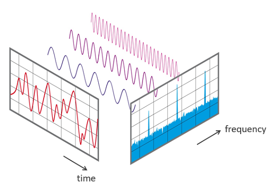
Each sound wave will be represented by its spectrum, and digitally it may be computed utilizing the Fast Fourier Transform (FFT).

A typical strategy to signify audio knowledge is to interrupt it into small chunks, which normally overlap. For every chunk we use the FFT to calculate the magnitude of the frequency spectrum. The spectra are then mixed, aspect by aspect, to type what we name a spectrogram.

It’s additionally frequent for speech recognition programs to additional rework the spectrum and compute the Mel-Frequency Cepstral Coefficients. This transformation takes under consideration that the human ear can’t discern the distinction between two intently spaced frequencies and well creates bins on the frequency axis. An ideal tutorial on MFCCs will be discovered here.

After this process, now we have a picture for every audio pattern and we will use convolutional neural networks, the usual structure kind in picture recognition fashions.

Downloading

First, let’s obtain knowledge to a listing in our mission. You’ll be able to both obtain from this link (~1GB) or from R with:

dir.create("knowledge")

download.file(
  url = "http://obtain.tensorflow.org/knowledge/speech_commands_v0.01.tar.gz", 
  destfile = "knowledge/speech_commands_v0.01.tar.gz"
)

untar("knowledge/speech_commands_v0.01.tar.gz", exdir = "knowledge/speech_commands_v0.01")

Contained in the knowledge listing we can have a folder referred to as speech_commands_v0.01. The WAV audio information inside this listing are organised in sub-folders with the label names. For instance, all one-second audio information of individuals talking the phrase “mattress” are contained in the mattress listing. There are 30 of them and a particular one referred to as _background_noise_ which comprises varied patterns that might be blended in to simulate background noise.

Importing

On this step we’ll record all audio .wav information right into a tibble with 3 columns:

• fname: the file identify;
• class: the label for every audio file;
• class_id: a singular integer quantity ranging from zero for every class – used to one-hot encode the lessons.

This might be helpful to the following step after we will create a generator utilizing the tfdatasets package deal.

Generator

We’ll now create our Dataset, which within the context of tfdatasets, provides operations to the TensorFlow graph as a way to learn and pre-process knowledge. Since they’re TensorFlow ops, they’re executed in C++ and in parallel with mannequin coaching.

The generator we’ll create might be accountable for studying the audio information from disk, creating the spectrogram for every one and batching the outputs.

Let’s begin by creating the dataset from slices of the knowledge.body with audio file names and lessons we simply created.

Now, let’s outline the parameters for spectrogram creation. We have to outline window_size_ms which is the scale in milliseconds of every chunk we’ll break the audio wave into, and window_stride_ms, the space between the facilities of adjoining chunks:

window_size_ms <- 30
window_stride_ms <- 10

Now we’ll convert the window measurement and stride from milliseconds to samples. We’re contemplating that our audio information have 16,000 samples per second (1000 ms).

window_size <- as.integer(16000*window_size_ms/1000)
stride <- as.integer(16000*window_stride_ms/1000)

We’ll receive different portions that might be helpful for spectrogram creation, just like the variety of chunks and the FFT measurement, i.e., the variety of bins on the frequency axis. The operate we’re going to use to compute the spectrogram doesn’t permit us to vary the FFT measurement and as an alternative by default makes use of the primary energy of two better than the window measurement.

We’ll now use dataset_map which permits us to specify a pre-processing operate for every statement (line) of our dataset. It’s on this step that we learn the uncooked audio file from disk and create its spectrogram and the one-hot encoded response vector.

# shortcuts to used TensorFlow modules.
audio_ops <- tf$contrib$framework$python$ops$audio_ops

ds <- ds %>%
  dataset_map(operate(obs) {
    
    # a great way to debug when constructing tfdatsets pipelines is to make use of a print
    # assertion like this:
    # print(str(obs))
    
    # decoding wav information
    audio_binary <- tf$read_file(tf$reshape(obs$fname, form = list()))
    wav <- audio_ops$decode_wav(audio_binary, desired_channels = 1)
    
    # create the spectrogram
    spectrogram <- audio_ops$audio_spectrogram(
      wav$audio, 
      window_size = window_size, 
      stride = stride,
      magnitude_squared = TRUE
    )
    
    # normalization
    spectrogram <- tf$log(tf$abs(spectrogram) + 0.01)
    
    # transferring channels to final dim
    spectrogram <- tf$transpose(spectrogram, perm = c(1L, 2L, 0L))
    
    # rework the class_id right into a one-hot encoded vector
    response <- tf$one_hot(obs$class_id, 30L)
    
    list(spectrogram, response)
  }) 

Now, we’ll specify how we wish batch observations from the dataset. We’re utilizing dataset_shuffle since we need to shuffle observations from the dataset, in any other case it will comply with the order of the df object. Then we use dataset_repeat as a way to inform TensorFlow that we need to preserve taking observations from the dataset even when all observations have already been used. And most significantly right here, we use dataset_padded_batch to specify that we wish batches of measurement 32, however they need to be padded, ie. if some statement has a unique measurement we pad it with zeroes. The padded form is handed to dataset_padded_batch through the padded_shapes argument and we use NULL to state that this dimension doesn’t must be padded.

ds <- ds %>% 
  dataset_shuffle(buffer_size = 100) %>%
  dataset_repeat() %>%
  dataset_padded_batch(
    batch_size = 32, 
    padded_shapes = list(
      form(n_chunks, fft_size, NULL), 
      form(NULL)
    )
  )

That is our dataset specification, however we would wish to rewrite all of the code for the validation knowledge, so it’s good follow to wrap this right into a operate of the information and different essential parameters like window_size_ms and window_stride_ms. Under, we’ll outline a operate referred to as data_generator that can create the generator relying on these inputs.

data_generator <- operate(df, batch_size, shuffle = TRUE, 
                           window_size_ms = 30, window_stride_ms = 10) {
  
  window_size <- as.integer(16000*window_size_ms/1000)
  stride <- as.integer(16000*window_stride_ms/1000)
  fft_size <- as.integer(2^trunc(log(window_size, 2)) + 1)
  n_chunks <- length(seq(window_size/2, 16000 - window_size/2, stride))
  
  ds <- tensor_slices_dataset(df)
  
  if (shuffle) 
    ds <- ds %>% dataset_shuffle(buffer_size = 100)  
  
  ds <- ds %>%
    dataset_map(operate(obs) {
      
      # decoding wav information
      audio_binary <- tf$read_file(tf$reshape(obs$fname, form = list()))
      wav <- audio_ops$decode_wav(audio_binary, desired_channels = 1)
      
      # create the spectrogram
      spectrogram <- audio_ops$audio_spectrogram(
        wav$audio, 
        window_size = window_size, 
        stride = stride,
        magnitude_squared = TRUE
      )
      
      spectrogram <- tf$log(tf$abs(spectrogram) + 0.01)
      spectrogram <- tf$transpose(spectrogram, perm = c(1L, 2L, 0L))
      
      # rework the class_id right into a one-hot encoded vector
      response <- tf$one_hot(obs$class_id, 30L)
      
      list(spectrogram, response)
    }) %>%
    dataset_repeat()
  
  ds <- ds %>% 
    dataset_padded_batch(batch_size, list(form(n_chunks, fft_size, NULL), form(NULL)))
  
  ds
}

Now, we will outline coaching and validation knowledge mills. It’s price noting that executing this received’t truly compute any spectrogram or learn any file. It’ll solely outline within the TensorFlow graph the way it ought to learn and pre-process knowledge.

set.seed(6)
id_train <- sample(nrow(df), measurement = 0.7*nrow(df))

ds_train <- data_generator(
  df[id_train,], 
  batch_size = 32, 
  window_size_ms = 30, 
  window_stride_ms = 10
)
ds_validation <- data_generator(
  df[-id_train,], 
  batch_size = 32, 
  shuffle = FALSE, 
  window_size_ms = 30, 
  window_stride_ms = 10
)

To really get a batch from the generator we might create a TensorFlow session and ask it to run the generator. For instance:

sess <- tf$Session()
batch <- next_batch(ds_train)
str(sess$run(batch))

Checklist of two
 $ : num [1:32, 1:98, 1:257, 1] -4.6 -4.6 -4.61 -4.6 -4.6 ...
 $ : num [1:32, 1:30] 0 0 0 0 0 0 0 0 0 0 ...

Every time you run sess$run(batch) you must see a unique batch of observations.

Mannequin definition

Now that we all know how we’ll feed our knowledge we will concentrate on the mannequin definition. The spectrogram will be handled like a picture, so architectures which might be generally utilized in picture recognition duties ought to work nicely with the spectrograms too.

We’ll construct a convolutional neural community much like what now we have constructed here for the MNIST dataset.

The enter measurement is outlined by the variety of chunks and the FFT measurement. Like we defined earlier, they are often obtained from the window_size_ms and window_stride_ms used to generate the spectrogram.

We’ll now outline our mannequin utilizing the Keras sequential API:

mannequin <- keras_model_sequential()
mannequin %>%  
  layer_conv_2d(input_shape = c(n_chunks, fft_size, 1), 
                filters = 32, kernel_size = c(3,3), activation = 'relu') %>% 
  layer_max_pooling_2d(pool_size = c(2, 2)) %>% 
  layer_conv_2d(filters = 64, kernel_size = c(3,3), activation = 'relu') %>% 
  layer_max_pooling_2d(pool_size = c(2, 2)) %>% 
  layer_conv_2d(filters = 128, kernel_size = c(3,3), activation = 'relu') %>% 
  layer_max_pooling_2d(pool_size = c(2, 2)) %>% 
  layer_conv_2d(filters = 256, kernel_size = c(3,3), activation = 'relu') %>% 
  layer_max_pooling_2d(pool_size = c(2, 2)) %>% 
  layer_dropout(fee = 0.25) %>% 
  layer_flatten() %>% 
  layer_dense(items = 128, activation = 'relu') %>% 
  layer_dropout(fee = 0.5) %>% 
  layer_dense(items = 30, activation = 'softmax')

We used 4 layers of convolutions mixed with max pooling layers to extract options from the spectrogram photos and a pair of dense layers on the prime. Our community is relatively easy when in comparison with extra superior architectures like ResNet or DenseNet that carry out very nicely on picture recognition duties.

Now let’s compile our mannequin. We’ll use categorical cross entropy because the loss operate and use the Adadelta optimizer. It’s additionally right here that we outline that we’ll take a look at the accuracy metric throughout coaching.

mannequin %>% compile(
  loss = loss_categorical_crossentropy,
  optimizer = optimizer_adadelta(),
  metrics = c('accuracy')
)

Mannequin becoming

Now, we’ll match our mannequin. In Keras we will use TensorFlow Datasets as inputs to the fit_generator operate and we’ll do it right here.

mannequin %>% fit_generator(
  generator = ds_train,
  steps_per_epoch = 0.7*nrow(df)/32,
  epochs = 10, 
  validation_data = ds_validation, 
  validation_steps = 0.3*nrow(df)/32
)

Epoch 1/10
1415/1415 [==============================] - 87s 62ms/step - loss: 2.0225 - acc: 0.4184 - val_loss: 0.7855 - val_acc: 0.7907
Epoch 2/10
1415/1415 [==============================] - 75s 53ms/step - loss: 0.8781 - acc: 0.7432 - val_loss: 0.4522 - val_acc: 0.8704
Epoch 3/10
1415/1415 [==============================] - 75s 53ms/step - loss: 0.6196 - acc: 0.8190 - val_loss: 0.3513 - val_acc: 0.9006
Epoch 4/10
1415/1415 [==============================] - 75s 53ms/step - loss: 0.4958 - acc: 0.8543 - val_loss: 0.3130 - val_acc: 0.9117
Epoch 5/10
1415/1415 [==============================] - 75s 53ms/step - loss: 0.4282 - acc: 0.8754 - val_loss: 0.2866 - val_acc: 0.9213
Epoch 6/10
1415/1415 [==============================] - 76s 53ms/step - loss: 0.3852 - acc: 0.8885 - val_loss: 0.2732 - val_acc: 0.9252
Epoch 7/10
1415/1415 [==============================] - 75s 53ms/step - loss: 0.3566 - acc: 0.8991 - val_loss: 0.2700 - val_acc: 0.9269
Epoch 8/10
1415/1415 [==============================] - 76s 54ms/step - loss: 0.3364 - acc: 0.9045 - val_loss: 0.2573 - val_acc: 0.9284
Epoch 9/10
1415/1415 [==============================] - 76s 53ms/step - loss: 0.3220 - acc: 0.9087 - val_loss: 0.2537 - val_acc: 0.9323
Epoch 10/10
1415/1415 [==============================] - 76s 54ms/step - loss: 0.2997 - acc: 0.9150 - val_loss: 0.2582 - val_acc: 0.9323

The mannequin’s accuracy is 93.23%. Let’s discover ways to make predictions and try the confusion matrix.

Making predictions

We will use thepredict_generator operate to make predictions on a brand new dataset. Let’s make predictions for our validation dataset.
The predict_generator operate wants a step argument which is the variety of instances the generator might be referred to as.

We will calculate the variety of steps by figuring out the batch measurement, and the scale of the validation dataset.

df_validation <- df[-id_train,]
n_steps <- nrow(df_validation)/32 + 1

We will then use the predict_generator operate:

predictions <- predict_generator(
  mannequin, 
  ds_validation, 
  steps = n_steps
  )
str(predictions)

num [1:19424, 1:30] 1.22e-13 7.30e-19 5.29e-10 6.66e-22 1.12e-17 ...

It will output a matrix with 30 columns – one for every phrase and n_steps*batch_size variety of rows. Be aware that it begins repeating the dataset on the finish to create a full batch.

We will compute the anticipated class by taking the column with the best chance, for instance.

lessons <- apply(predictions, 1, which.max) - 1

A pleasant visualization of the confusion matrix is to create an alluvial diagram:

library(dplyr)
library(alluvial)
x <- df_validation %>%
  mutate(pred_class_id = head(lessons, nrow(df_validation))) %>%
  left_join(
    df_validation %>% distinct(class_id, class) %>% rename(pred_class = class),
    by = c("pred_class_id" = "class_id")
  ) %>%
  mutate(right = pred_class == class) %>%
  count(pred_class, class, right)

alluvial(
  x %>% select(class, pred_class),
  freq = x$n,
  col = ifelse(x$right, "lightblue", "pink"),
  border = ifelse(x$right, "lightblue", "pink"),
  alpha = 0.6,
  conceal = x$n < 20
)

We will see from the diagram that probably the most related mistake our mannequin makes is to categorise “tree” as “three”. There are different frequent errors like classifying “go” as “no”, “up” as “off”. At 93% accuracy for 30 lessons, and contemplating the errors we will say that this mannequin is fairly affordable.

The saved mannequin occupies 25Mb of disk area, which is cheap for a desktop however is probably not on small units. We might practice a smaller mannequin, with fewer layers, and see how a lot the efficiency decreases.

In speech recognition duties its additionally frequent to do some type of knowledge augmentation by mixing a background noise to the spoken audio, making it extra helpful for actual functions the place it’s frequent to produce other irrelevant sounds taking place within the atmosphere.

The complete code to breed this tutorial is offered here.