Posit AI Weblog: Picture-to-image translation with pix2pix
What do we have to practice a neural community? A typical reply is: a mannequin, a value perform, and an optimization algorithm.
(I do know: I’m leaving out crucial factor right here – the information.)
As laptop applications work with numbers, the fee perform must be fairly particular: We are able to’t simply say predict subsequent month’s demand for garden mowers please, and do your greatest, we now have to say one thing like this: Reduce the squared deviation of the estimate from the goal worth.
In some instances it might be easy to map a activity to a measure of error, in others, it might not. Take into account the duty of producing non-existing objects of a sure sort (like a face, a scene, or a video clip). How can we quantify success?
The trick with generative adversarial networks (GANs) is to let the community be taught the fee perform.
As proven in Generating images with Keras and TensorFlow eager execution, in a easy GAN the setup is that this: One agent, the generator, retains on producing faux objects. The opposite, the discriminator, is tasked to inform aside the true objects from the faux ones. For the generator, loss is augmented when its fraud will get found, that means that the generator’s price perform depends upon what the discriminator does. For the discriminator, loss grows when it fails to appropriately inform aside generated objects from genuine ones.
In a GAN of the sort simply described, creation begins from white noise. Nonetheless in the true world, what’s required could also be a type of transformation, not creation. Take, for instance, colorization of black-and-white photographs, or conversion of aerials to maps. For purposes like these, we situation on extra enter: Therefore the title, conditional adversarial networks.
Put concretely, this implies the generator is handed not (or not solely) white noise, however knowledge of a sure enter construction, similar to edges or shapes. It then has to generate realistic-looking footage of actual objects having these shapes.
The discriminator, too, could obtain the shapes or edges as enter, along with the faux and actual objects it’s tasked to inform aside.
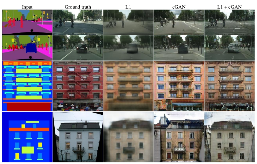
Listed below are a number of examples of conditioning, taken from the paper we’ll be implementing (see under):

On this put up, we port to R a Google Colaboratory Notebook utilizing Keras with keen execution. We’re implementing the essential structure from pix2pix, as described by Isola et al. of their 2016 paper(Isola et al. 2016). It’s an attention-grabbing paper to learn because it validates the method on a bunch of various datasets, and shares outcomes of utilizing totally different loss households, too:

Conditions
The code proven right here will work with the present CRAN variations of tensorflow, keras, and tfdatasets. Additionally, be sure you test that you simply’re utilizing no less than model 1.9 of TensorFlow. If that isn’t the case, as of this writing, this
will get you model 1.10.
When loading libraries, please be sure you’re executing the primary 4 traces within the precise order proven. We’d like to verify we’re utilizing the TensorFlow implementation of Keras (tf.keras in Python land), and we now have to allow keen execution earlier than utilizing TensorFlow in any means.
No have to copy-paste any code snippets – you’ll discover the whole code (so as vital for execution) right here: eager-pix2pix.R.
Dataset
For this put up, we’re working with one of many datasets used within the paper, a preprocessed model of the CMP Facade Dataset.
Pictures comprise the bottom reality – that we’d want for the generator to generate, and for the discriminator to appropriately detect as genuine – and the enter we’re conditioning on (a rough segmention into object courses) subsequent to one another in the identical file.

Preprocessing
Clearly, our preprocessing must break up the enter photographs into components. That’s the very first thing that occurs within the perform under.
After that, motion depends upon whether or not we’re within the coaching or testing phases. If we’re coaching, we carry out random jittering, by way of upsizing the picture to 286x286 after which cropping to the unique measurement of 256x256. In about 50% of the instances, we additionally flipping the picture left-to-right.
In each instances, coaching and testing, we normalize the picture to the vary between -1 and 1.
Be aware using the tf$picture module for picture -related operations. That is required as the pictures might be streamed by way of tfdatasets, which works on TensorFlow graphs.
img_width <- 256L
img_height <- 256L

load_image <- perform(image_file, is_train) {

  picture <- tf$read_file(image_file)
  picture <- tf$picture$decode_jpeg(picture)

  w <- as.integer(k_shape(picture)[2])
  w2 <- as.integer(w / 2L)
  real_image <- picture[ , 1L:w2, ]
  input_image <- picture[ , (w2 + 1L):w, ]

  input_image <- k_cast(input_image, tf$float32)
  real_image <- k_cast(real_image, tf$float32)

  if (is_train) {
    input_image <-
      tf$picture$resize_images(input_image,
                             c(286L, 286L),
                             align_corners = TRUE,
                             technique = 2)
    real_image <- tf$picture$resize_images(real_image,
                                         c(286L, 286L),
                                         align_corners = TRUE,
                                         technique = 2)

    stacked_image <-
      k_stack(list(input_image, real_image), axis = 1)
    cropped_image <-
      tf$random_crop(stacked_image, measurement = c(2L, img_height, img_width, 3L))
    c(input_image, real_image) %<-%
      list(cropped_image[1, , , ], cropped_image[2, , , ])

    if (runif(1) > 0.5) {
      input_image <- tf$picture$flip_left_right(input_image)
      real_image <- tf$picture$flip_left_right(real_image)
    }

  } else {
    input_image <-
      tf$picture$resize_images(
        input_image,
        measurement = c(img_height, img_width),
        align_corners = TRUE,
        technique = 2
      )
    real_image <-
      tf$picture$resize_images(
        real_image,
        measurement = c(img_height, img_width),
        align_corners = TRUE,
        technique = 2
      )
  }

  input_image <- (input_image / 127.5) - 1
  real_image <- (real_image / 127.5) - 1

  list(input_image, real_image)
}
Streaming the information
The pictures might be streamed by way of tfdatasets, utilizing a batch measurement of 1.
Be aware how the load_image perform we outlined above is wrapped in tf$py_func to allow accessing tensor values within the traditional keen means (which by default, as of this writing, is just not doable with the TensorFlow datasets API).
# change to the place you unpacked the information
# there might be practice, val and take a look at subdirectories under
data_dir <- "facades"

buffer_size <- 400
batch_size <- 1
batches_per_epoch <- buffer_size / batch_size

train_dataset <-
  tf$knowledge$Dataset$list_files(file.path(data_dir, "practice/*.jpg")) %>%
  dataset_shuffle(buffer_size) %>%
  dataset_map(perform(picture) {
    tf$py_func(load_image, list(picture, TRUE), list(tf$float32, tf$float32))
  }) %>%
  dataset_batch(batch_size)

test_dataset <-
  tf$knowledge$Dataset$list_files(file.path(data_dir, "take a look at/*.jpg")) %>%
  dataset_map(perform(picture) {
    tf$py_func(load_image, list(picture, TRUE), list(tf$float32, tf$float32))
  }) %>%
  dataset_batch(batch_size)
Defining the actors
Generator
First, right here’s the generator. Let’s begin with a birds-eye view.
The generator receives as enter a rough segmentation, of measurement 256×256, and may produce a pleasant shade picture of a facade.
It first successively downsamples the enter, as much as a minimal measurement of 1×1. Then after maximal condensation, it begins upsampling once more, till it has reached the required output decision of 256×256.
Throughout downsampling, as spatial decision decreases, the variety of filters will increase. Throughout upsampling, it goes the other means.
generator <- perform(title = "generator") {

  keras_model_custom(title = title, perform(self) {

    self$down1 <- downsample(64, 4, apply_batchnorm = FALSE)
    self$down2 <- downsample(128, 4)
    self$down3 <- downsample(256, 4)
    self$down4 <- downsample(512, 4)
    self$down5 <- downsample(512, 4)
    self$down6 <- downsample(512, 4)
    self$down7 <- downsample(512, 4)
    self$down8 <- downsample(512, 4)

    self$up1 <- upsample(512, 4, apply_dropout = TRUE)
    self$up2 <- upsample(512, 4, apply_dropout = TRUE)
    self$up3 <- upsample(512, 4, apply_dropout = TRUE)
    self$up4 <- upsample(512, 4)
    self$up5 <- upsample(256, 4)
    self$up6 <- upsample(128, 4)
    self$up7 <- upsample(64, 4)

    self$final <- layer_conv_2d_transpose(
      filters = 3,
      kernel_size = 4,
      strides = 2,
      padding = "similar",
      kernel_initializer = initializer_random_normal(0, 0.2),
      activation = "tanh"
    )

    perform(x, masks = NULL, coaching = TRUE) {           # x form == (bs, 256, 256, 3)

      x1 <- x %>% self$down1(coaching = coaching)         # (bs, 128, 128, 64)
      x2 <- self$down2(x1, coaching = coaching)           # (bs, 64, 64, 128)
      x3 <- self$down3(x2, coaching = coaching)           # (bs, 32, 32, 256)
      x4 <- self$down4(x3, coaching = coaching)           # (bs, 16, 16, 512)
      x5 <- self$down5(x4, coaching = coaching)           # (bs, 8, 8, 512)
      x6 <- self$down6(x5, coaching = coaching)           # (bs, 4, 4, 512)
      x7 <- self$down7(x6, coaching = coaching)           # (bs, 2, 2, 512)
      x8 <- self$down8(x7, coaching = coaching)           # (bs, 1, 1, 512)

      x9 <- self$up1(list(x8, x7), coaching = coaching)   # (bs, 2, 2, 1024)
      x10 <- self$up2(list(x9, x6), coaching = coaching)  # (bs, 4, 4, 1024)
      x11 <- self$up3(list(x10, x5), coaching = coaching) # (bs, 8, 8, 1024)
      x12 <- self$up4(list(x11, x4), coaching = coaching) # (bs, 16, 16, 1024)
      x13 <- self$up5(list(x12, x3), coaching = coaching) # (bs, 32, 32, 512)
      x14 <- self$up6(list(x13, x2), coaching = coaching) # (bs, 64, 64, 256)
      x15 <-self$up7(list(x14, x1), coaching = coaching)  # (bs, 128, 128, 128)
      x16 <- self$final(x15)                               # (bs, 256, 256, 3)
      x16
    }
  })
}
How can spatial info be preserved if we downsample all the way in which all the way down to a single pixel? The generator follows the overall precept of a U-Web (Ronneberger, Fischer, and Brox 2015), the place skip connections exist from layers earlier within the downsampling course of to layers in a while the way in which up.

Let’s take the road
x15 <-self$up7(list(x14, x1), coaching = coaching)from the name technique.
Right here, the inputs to self$up are x14, which went by the entire down- and upsampling, and x1, the output from the very first downsampling step. The previous has decision 64×64, the latter, 128×128. How do they get mixed?
That’s taken care of by upsample, technically a customized mannequin of its personal.
As an apart, we comment how customized fashions allow you to pack your code into good, reusable modules.
upsample <- perform(filters,
                     measurement,
                     apply_dropout = FALSE,
                     title = "upsample") {

  keras_model_custom(title = NULL, perform(self) {

    self$apply_dropout <- apply_dropout
    self$up_conv <- layer_conv_2d_transpose(
      filters = filters,
      kernel_size = measurement,
      strides = 2,
      padding = "similar",
      kernel_initializer = initializer_random_normal(),
      use_bias = FALSE
    )
    self$batchnorm <- layer_batch_normalization()
    if (self$apply_dropout) {
      self$dropout <- layer_dropout(charge = 0.5)
    }

    perform(xs, masks = NULL, coaching = TRUE) {

      c(x1, x2) %<-% xs
      x <- self$up_conv(x1) %>% self$batchnorm(coaching = coaching)
      if (self$apply_dropout) {
        x %>% self$dropout(coaching = coaching)
      }
      x %>% layer_activation("relu")
      concat <- k_concatenate(list(x, x2))
      concat
    }
  })
}
x14 is upsampled to double its measurement, and x1 is appended as is.
The axis of concatenation right here is axis 4, the function map / channels axis. x1 comes with 64 channels, x14 comes out of layer_conv_2d_transpose with 64 channels, too (as a result of self$up7 has been outlined that means). So we find yourself with a picture of decision 128×128 and 128 function maps for the output of step x15.
Downsampling, too, is factored out to its personal mannequin. Right here too, the variety of filters is configurable.
downsample <- perform(filters,
                       measurement,
                       apply_batchnorm = TRUE,
                       title = "downsample") {

  keras_model_custom(title = title, perform(self) {

    self$apply_batchnorm <- apply_batchnorm
    self$conv1 <- layer_conv_2d(
      filters = filters,
      kernel_size = measurement,
      strides = 2,
      padding = 'similar',
      kernel_initializer = initializer_random_normal(0, 0.2),
      use_bias = FALSE
    )
    if (self$apply_batchnorm) {
      self$batchnorm <- layer_batch_normalization()
    }

    perform(x, masks = NULL, coaching = TRUE) {

      x <- self$conv1(x)
      if (self$apply_batchnorm) {
        x %>% self$batchnorm(coaching = coaching)
      }
      x %>% layer_activation_leaky_relu()
    }
  })
}
Now for the discriminator.
Discriminator
Once more, let’s begin with a birds-eye view.
The discriminator receives as enter each the coarse segmentation and the bottom reality. Each are concatenated and processed collectively. Similar to the generator, the discriminator is thus conditioned on the segmentation.
What does the discriminator return? The output of self$final has one channel, however a spatial decision of 30×30: We’re outputting a likelihood for every of 30×30 picture patches (which is why the authors are calling this a PatchGAN).
The discriminator thus engaged on small picture patches means it solely cares about native construction, and consequently, enforces correctness within the excessive frequencies solely. Correctness within the low frequencies is taken care of by a further L1 element within the discriminator loss that operates over the entire picture (as we’ll see under).
discriminator <- perform(title = "discriminator") {

  keras_model_custom(title = title, perform(self) {

    self$down1 <- disc_downsample(64, 4, FALSE)
    self$down2 <- disc_downsample(128, 4)
    self$down3 <- disc_downsample(256, 4)
    self$zero_pad1 <- layer_zero_padding_2d()
    self$conv <- layer_conv_2d(
      filters = 512,
      kernel_size = 4,
      strides = 1,
      kernel_initializer = initializer_random_normal(),
      use_bias = FALSE
    )
    self$batchnorm <- layer_batch_normalization()
    self$zero_pad2 <- layer_zero_padding_2d()
    self$final <- layer_conv_2d(
      filters = 1,
      kernel_size = 4,
      strides = 1,
      kernel_initializer = initializer_random_normal()
    )

    perform(x, y, masks = NULL, coaching = TRUE) {

      x <- k_concatenate(list(x, y)) %>%            # (bs, 256, 256, channels*2)
        self$down1(coaching = coaching) %>%         # (bs, 128, 128, 64)
        self$down2(coaching = coaching) %>%         # (bs, 64, 64, 128)
        self$down3(coaching = coaching) %>%         # (bs, 32, 32, 256)
        self$zero_pad1() %>%                        # (bs, 34, 34, 256)
        self$conv() %>%                             # (bs, 31, 31, 512)
        self$batchnorm(coaching = coaching) %>%
        layer_activation_leaky_relu() %>%
        self$zero_pad2() %>%                        # (bs, 33, 33, 512)
        self$final()                                 # (bs, 30, 30, 1)
      x
    }
  })
}
And right here’s the factored-out downsampling performance, once more offering the means to configure the variety of filters.
disc_downsample <- perform(filters,
                            measurement,
                            apply_batchnorm = TRUE,
                            title = "disc_downsample") {

  keras_model_custom(title = title, perform(self) {

    self$apply_batchnorm <- apply_batchnorm
    self$conv1 <- layer_conv_2d(
      filters = filters,
      kernel_size = measurement,
      strides = 2,
      padding = 'similar',
      kernel_initializer = initializer_random_normal(0, 0.2),
      use_bias = FALSE
    )
    if (self$apply_batchnorm) {
      self$batchnorm <- layer_batch_normalization()
    }

    perform(x, masks = NULL, coaching = TRUE) {
      x <- self$conv1(x)
      if (self$apply_batchnorm) {
        x %>% self$batchnorm(coaching = coaching)
      }
      x %>% layer_activation_leaky_relu()
    }
  })
}
Losses and optimizer
As we stated within the introduction, the concept of a GAN is to have the community be taught the fee perform.
Extra concretely, the factor it ought to be taught is the steadiness between two losses, the generator loss and the discriminator loss.
Every of them individually, in fact, must be supplied with a loss perform, so there are nonetheless choices to be made.
For the generator, two issues issue into the loss: First, does the discriminator debunk my creations as faux?
Second, how massive is absolutely the deviation of the generated picture from the goal?
The latter issue doesn’t should be current in a conditional GAN, however was included by the authors to additional encourage proximity to the goal, and empirically discovered to ship higher outcomes.
lambda <- 100 # worth chosen by the authors of the paper
generator_loss <- perform(disc_judgment, generated_output, goal) {
    gan_loss <- tf$losses$sigmoid_cross_entropy(
      tf$ones_like(disc_judgment),
      disc_judgment
    )
    l1_loss <- tf$reduce_mean(tf$abs(goal - generated_output))
    gan_loss + (lambda * l1_loss)
  }
The discriminator loss seems to be as in a typical (un-conditional) GAN. Its first element is decided by how precisely it classifies actual photographs as actual, whereas the second depends upon its competence in judging faux photographs as faux.
discriminator_loss <- perform(real_output, generated_output) {
  real_loss <- tf$losses$sigmoid_cross_entropy(
    multi_class_labels = tf$ones_like(real_output),
    logits = real_output
  )
  generated_loss <- tf$losses$sigmoid_cross_entropy(
    multi_class_labels = tf$zeros_like(generated_output),
    logits = generated_output
  )
  real_loss + generated_loss
}
For optimization, we depend on Adam for each the generator and the discriminator.
discriminator_optimizer <- tf$practice$AdamOptimizer(2e-4, beta1 = 0.5)
generator_optimizer <- tf$practice$AdamOptimizer(2e-4, beta1 = 0.5)
The sport
We’re able to have the generator and the discriminator play the sport!
Under, we use defun to compile the respective R capabilities into TensorFlow graphs, to hurry up computations.
generator <- generator()
discriminator <- discriminator()

generator$name = tf$contrib$keen$defun(generator$name)
discriminator$name = tf$contrib$keen$defun(discriminator$name)
We additionally create a tf$practice$Checkpoint object that can permit us to avoid wasting and restore coaching weights.
checkpoint_dir <- "./checkpoints_pix2pix"
checkpoint_prefix <- file.path(checkpoint_dir, "ckpt")
checkpoint <- tf$practice$Checkpoint(
    generator_optimizer = generator_optimizer,
    discriminator_optimizer = discriminator_optimizer,
    generator = generator,
    discriminator = discriminator
)
Coaching is a loop over epochs with an internal loop over batches yielded by the dataset.
As traditional with keen execution, tf$GradientTape takes care of recording the ahead cross and figuring out the gradients, whereas the optimizer – there are two of them on this setup – adjusts the networks’ weights.
Each tenth epoch, we save the weights, and inform the generator to have a go on the first instance of the take a look at set, so we are able to monitor community progress. See generate_images within the companion code for this performance.
practice <- perform(dataset, num_epochs) {

  for (epoch in 1:num_epochs) {
    total_loss_gen <- 0
    total_loss_disc <- 0
    iter <- make_iterator_one_shot(train_dataset)

    until_out_of_range({
      batch <- iterator_get_next(iter)
      input_image <- batch[[1]]
      goal <- batch[[2]]

      with(tf$GradientTape() %as% gen_tape, {
        with(tf$GradientTape() %as% disc_tape, {

          gen_output <- generator(input_image, coaching = TRUE)
          disc_real_output <-
            discriminator(input_image, goal, coaching = TRUE)
          disc_generated_output <-
            discriminator(input_image, gen_output, coaching = TRUE)
          gen_loss <-
            generator_loss(disc_generated_output, gen_output, goal)
          disc_loss <-
            discriminator_loss(disc_real_output, disc_generated_output)
          total_loss_gen <- total_loss_gen + gen_loss
          total_loss_disc <- total_loss_disc + disc_loss
        })
      })

      generator_gradients <- gen_tape$gradient(gen_loss,
                                               generator$variables)
      discriminator_gradients <- disc_tape$gradient(disc_loss,
                                                    discriminator$variables)

      generator_optimizer$apply_gradients(transpose(list(
        generator_gradients,
        generator$variables
      )))
      discriminator_optimizer$apply_gradients(transpose(
        list(discriminator_gradients,
             discriminator$variables)
      ))

    })

    cat("Epoch ", epoch, "n")
    cat("Generator loss: ",
        total_loss_gen$numpy() / batches_per_epoch,
        "n")
    cat("Discriminator loss: ",
        total_loss_disc$numpy() / batches_per_epoch,
        "nn")

    if (epoch %% 10 == 0) {
      test_iter <- make_iterator_one_shot(test_dataset)
      batch <- iterator_get_next(test_iter)
      enter <- batch[[1]]
      goal <- batch[[2]]
      generate_images(generator, enter, goal, paste0("epoch_", i))
    }

    if (epoch %% 10 == 0) {
      checkpoint$save(file_prefix = checkpoint_prefix)
    }
  }
}

if (!restore) {
  practice(train_dataset, 200)
}
The outcomes
What has the community realized?
Right here’s a fairly typical end result from the take a look at set. It doesn’t look so dangerous.

Right here’s one other one. Curiously, the colours used within the faux picture match the earlier one’s fairly properly, although we used a further L1 loss to penalize deviations from the unique.

This decide from the take a look at set once more exhibits comparable hues, and it would already convey an impression one will get when going by the whole take a look at set: The community has not simply realized some steadiness between creatively turning a rough masks into an in depth picture on the one hand, and reproducing a concrete instance alternatively. It additionally has internalized the principle architectural fashion current within the dataset.

For an excessive instance, take this. The masks leaves an infinite lot of freedom, whereas the goal picture is a fairly untypical (maybe essentially the most untypical) decide from the take a look at set. The result is a construction that would characterize a constructing, or a part of a constructing, of particular texture and shade shades.

Conclusion
Once we say the community has internalized the dominant fashion of the coaching set, is that this a nasty factor? (We’re used to considering when it comes to overfitting on the coaching set.)
With GANs although, one may say all of it depends upon the aim. If it doesn’t match our objective, one factor we may strive is coaching on a number of datasets on the similar time.
Once more relying on what we wish to obtain, one other weak spot may very well be the shortage of stochasticity within the mannequin, as said by the authors of the paper themselves. This might be exhausting to keep away from when working with paired datasets as those utilized in pix2pix. An attention-grabbing various is CycleGAN(Zhu et al. 2017) that allows you to switch fashion between full datasets with out utilizing paired situations:

Lastly closing on a extra technical word, you could have seen the outstanding checkerboard results within the above faux examples. This phenomenon (and methods to deal with it) is beautifully defined in a 2016 article on distill.pub (Odena, Dumoulin, and Olah 2016).
In our case, it can largely be attributable to using layer_conv_2d_transpose for upsampling.
As per the authors (Odena, Dumoulin, and Olah 2016), a greater various is upsizing adopted by padding and (customary) convolution.
Should you’re , it needs to be easy to switch the instance code to make use of tf$picture$resize_images (utilizing ResizeMethod.NEAREST_NEIGHBOR as really helpful by the authors), tf$pad and layer_conv2d.


