Posit AI Weblog: Illustration studying with MMD-VAE

Not too long ago, we confirmed how you can generate images utilizing generative adversarial networks (GANs). GANs might yield wonderful outcomes, however the contract there mainly is: what you see is what you get.
Generally this can be all we wish. In different circumstances, we could also be extra all for truly modelling a website. We don’t simply wish to generate realistic-looking samples – we wish our samples to be positioned at particular coordinates in area area.

For instance, think about our area to be the area of facial expressions. Then our latent area is likely to be conceived as two-dimensional: In accordance with underlying emotional states, expressions differ on a positive-negative scale. On the similar time, they differ in depth. Now if we skilled a VAE on a set of facial expressions adequately overlaying the ranges, and it did in actual fact “uncover” our hypothesized dimensions, we may then use it to generate previously-nonexisting incarnations of factors (faces, that’s) in latent area.

Variational autoencoders are just like probabilistic graphical fashions in that they assume a latent area that’s liable for the observations, however unobservable. They’re just like plain autoencoders in that they compress, after which decompress once more, the enter area. In distinction to plain autoencoders although, the essential level right here is to plan a loss perform that permits to acquire informative representations in latent area.

In a nutshell

In customary VAEs (Kingma and Welling 2013), the target is to maximise the proof decrease certain (ELBO):

[ELBO = E[log p(x|z)] – KL(q(z)||p(z))]

In plain phrases and expressed by way of how we use it in apply, the primary part is the reconstruction loss we additionally see in plain (non-variational) autoencoders. The second is the Kullback-Leibler divergence between a previous imposed on the latent area (sometimes, an ordinary regular distribution) and the illustration of latent area as discovered from the information.

A significant criticism relating to the standard VAE loss is that it ends in uninformative latent area. Alternate options embrace (beta)-VAE(Burgess et al. 2018), Data-VAE (Zhao, Song, and Ermon 2017), and extra. The MMD-VAE(Zhao, Song, and Ermon 2017) carried out beneath is a subtype of Data-VAE that as a substitute of creating every illustration in latent area as comparable as potential to the prior, coerces the respective distributions to be as shut as potential. Right here MMD stands for most imply discrepancy, a similarity measure for distributions based mostly on matching their respective moments. We clarify this in additional element beneath.

Our goal in the present day

On this submit, we’re first going to implement an ordinary VAE that strives to maximise the ELBO. Then, we evaluate its efficiency to that of an Data-VAE utilizing the MMD loss.

Our focus shall be on inspecting the latent areas and see if, and the way, they differ as a consequence of the optimization standards used.

The area we’re going to mannequin shall be glamorous (trend!), however for the sake of manageability, confined to dimension 28 x 28: We’ll compress and reconstruct photographs from the Fashion MNIST dataset that has been developed as a drop-in to MNIST.

A regular variational autoencoder

Seeing we haven’t used TensorFlow keen execution for some weeks, we’ll do the mannequin in an keen means.
For those who’re new to keen execution, don’t fear: As each new method, it wants some getting accustomed to, however you’ll rapidly discover that many duties are made simpler when you use it. A easy but full, template-like instance is out there as a part of the Keras documentation.

Setup and information preparation

As common, we begin by ensuring we’re utilizing the TensorFlow implementation of Keras and enabling keen execution. In addition to tensorflow and keras, we additionally load tfdatasets to be used in information streaming.

By the way in which: No have to copy-paste any of the beneath code snippets. The 2 approaches can be found amongst our Keras examples, particularly, as eager_cvae.R and mmd_cvae.R.

The info comes conveniently with keras, all we have to do is the same old normalization and reshaping.

trend <- dataset_fashion_mnist()

c(train_images, train_labels) %<-% trend$practice
c(test_images, test_labels) %<-% trend$check

train_x <- train_images %>%
  `/`(255) %>%
  k_reshape(c(60000, 28, 28, 1))

test_x <- test_images %>% `/`(255) %>%
  k_reshape(c(10000, 28, 28, 1))

What do we’d like the check set for, given we’re going to practice an unsupervised (a greater time period being: semi-supervised) mannequin? We’ll use it to see how (beforehand unknown) information factors cluster collectively in latent area.

Now put together for streaming the information to keras:

buffer_size <- 60000
batch_size <- 100
batches_per_epoch <- buffer_size / batch_size

train_dataset <- tensor_slices_dataset(train_x) %>%
  dataset_shuffle(buffer_size) %>%
  dataset_batch(batch_size)

test_dataset <- tensor_slices_dataset(test_x) %>%
  dataset_batch(10000)

Subsequent up is defining the mannequin.

Encoder-decoder mannequin

The mannequin actually is 2 fashions: the encoder and the decoder. As we’ll see shortly, in the usual model of the VAE there’s a third part in between, performing the so-called reparameterization trick.

The encoder is a custom model, comprised of two convolutional layers and a dense layer. It returns the output of the dense layer cut up into two components, one storing the imply of the latent variables, the opposite their variance.

latent_dim <- 2

encoder_model <- perform(identify = NULL) {
  
  keras_model_custom(identify = identify, perform(self) {
    self$conv1 <-
      layer_conv_2d(
        filters = 32,
        kernel_size = 3,
        strides = 2,
        activation = "relu"
      )
    self$conv2 <-
      layer_conv_2d(
        filters = 64,
        kernel_size = 3,
        strides = 2,
        activation = "relu"
      )
    self$flatten <- layer_flatten()
    self$dense <- layer_dense(items = 2 * latent_dim)
    
    perform (x, masks = NULL) {
      x %>%
        self$conv1() %>%
        self$conv2() %>%
        self$flatten() %>%
        self$dense() %>%
        tf$cut up(num_or_size_splits = 2L, axis = 1L) 
    }
  })
}

We select the latent area to be of dimension 2 – simply because that makes visualization straightforward.
With extra advanced information, you’ll most likely profit from selecting the next dimensionality right here.

So the encoder compresses actual information into estimates of imply and variance of the latent area.
We then “not directly” pattern from this distribution (the so-called reparameterization trick):

reparameterize <- perform(imply, logvar) {
  eps <- k_random_normal(form = imply$form, dtype = tf$float64)
  eps * k_exp(logvar * 0.5) + imply
}

The sampled values will function enter to the decoder, who will try to map them again to the unique area.
The decoder is mainly a sequence of transposed convolutions, upsampling till we attain a decision of 28×28.

decoder_model <- perform(identify = NULL) {
  
  keras_model_custom(identify = identify, perform(self) {
    
    self$dense <- layer_dense(items = 7 * 7 * 32, activation = "relu")
    self$reshape <- layer_reshape(target_shape = c(7, 7, 32))
    self$deconv1 <-
      layer_conv_2d_transpose(
        filters = 64,
        kernel_size = 3,
        strides = 2,
        padding = "similar",
        activation = "relu"
      )
    self$deconv2 <-
      layer_conv_2d_transpose(
        filters = 32,
        kernel_size = 3,
        strides = 2,
        padding = "similar",
        activation = "relu"
      )
    self$deconv3 <-
      layer_conv_2d_transpose(
        filters = 1,
        kernel_size = 3,
        strides = 1,
        padding = "similar"
      )
    
    perform (x, masks = NULL) {
      x %>%
        self$dense() %>%
        self$reshape() %>%
        self$deconv1() %>%
        self$deconv2() %>%
        self$deconv3()
    }
  })
}

Word how the ultimate deconvolution doesn’t have the sigmoid activation you may need anticipated. It is because we shall be utilizing tf$nn$sigmoid_cross_entropy_with_logits when calculating the loss.

Talking of losses, let’s examine them now.

Loss calculations

One strategy to implement the VAE loss is combining reconstruction loss (cross entropy, within the current case) and Kullback-Leibler divergence. In Keras, the latter is out there straight as loss_kullback_leibler_divergence.

Right here, we comply with a current Google Colaboratory notebook in batch-estimating the entire ELBO as a substitute (as a substitute of simply estimating reconstruction loss and computing the KL-divergence analytically):

[ELBO batch estimate = log p(x_{batch}|z_{sampled})+log p(z)−log q(z_{sampled}|x_{batch})]

Calculation of the traditional loglikelihood is packaged right into a perform so we will reuse it through the coaching loop.

normal_loglik <- perform(pattern, imply, logvar, reduce_axis = 2) {
  loglik <- k_constant(0.5, dtype = tf$float64) *
    (k_log(2 * k_constant(pi, dtype = tf$float64)) +
    logvar +
    k_exp(-logvar) * (pattern - imply) ^ 2)
  - k_sum(loglik, axis = reduce_axis)
}

Peeking forward some, throughout coaching we’ll compute the above as follows.

First,

crossentropy_loss <- tf$nn$sigmoid_cross_entropy_with_logits(
  logits = preds,
  labels = x
)
logpx_z <- - k_sum(crossentropy_loss)

yields (log p(x|z)), the loglikelihood of the reconstructed samples given values sampled from latent area (a.ok.a. reconstruction loss).

Then,

logpz <- normal_loglik(
  z,
  k_constant(0, dtype = tf$float64),
  k_constant(0, dtype = tf$float64)
)

offers (log p(z)), the prior loglikelihood of (z). The prior is assumed to be customary regular, as is most frequently the case with VAEs.

Lastly,

logqz_x <- normal_loglik(z, imply, logvar)

vields (log q(z|x)), the loglikelihood of the samples (z) given imply and variance computed from the noticed samples (x).

From these three parts, we’ll compute the ultimate loss as

loss <- -k_mean(logpx_z + logpz - logqz_x)

After this peaking forward, let’s rapidly end the setup so we prepare for coaching.

Ultimate setup

In addition to the loss, we’d like an optimizer that can try to decrease it.

optimizer <- tf$practice$AdamOptimizer(1e-4)

We instantiate our fashions …

encoder <- encoder_model()
decoder <- decoder_model()

and arrange checkpointing, so we will later restore skilled weights.

checkpoint_dir <- "./checkpoints_cvae"
checkpoint_prefix <- file.path(checkpoint_dir, "ckpt")
checkpoint <- tf$practice$Checkpoint(
  optimizer = optimizer,
  encoder = encoder,
  decoder = decoder
)

From the coaching loop, we’ll, in sure intervals, additionally name three capabilities not reproduced right here (however obtainable within the code example): generate_random_clothes, used to generate garments from random samples from the latent area; show_latent_space, that shows the entire check set in latent (2-dimensional, thus simply visualizable) area; and show_grid, that generates garments in response to enter values systematically spaced out in a grid.

Let’s begin coaching! Truly, earlier than we do this, let’s take a look at what these capabilities show earlier than any coaching: As a substitute of garments, we see random pixels. Latent area has no construction. And several types of garments don’t cluster collectively in latent area.

Coaching loop

We’re coaching for 50 epochs right here. For every epoch, we loop over the coaching set in batches. For every batch, we comply with the same old keen execution move: Contained in the context of a GradientTape, apply the mannequin and calculate the present loss; then outdoors this context calculate the gradients and let the optimizer carry out backprop.

What’s particular right here is that we have now two fashions that each want their gradients calculated and weights adjusted. This may be taken care of by a single gradient tape, supplied we create it persistent.

After every epoch, we save present weights and each ten epochs, we additionally save plots for later inspection.

num_epochs <- 50

for (epoch in seq_len(num_epochs)) {
  iter <- make_iterator_one_shot(train_dataset)
  
  total_loss <- 0
  logpx_z_total <- 0
  logpz_total <- 0
  logqz_x_total <- 0
  
  until_out_of_range({
    x <-  iterator_get_next(iter)
    
    with(tf$GradientTape(persistent = TRUE) %as% tape, {
      
      c(imply, logvar) %<-% encoder(x)
      z <- reparameterize(imply, logvar)
      preds <- decoder(z)
      
      crossentropy_loss <-
        tf$nn$sigmoid_cross_entropy_with_logits(logits = preds, labels = x)
      logpx_z <-
        - k_sum(crossentropy_loss)
      logpz <-
        normal_loglik(z,
                      k_constant(0, dtype = tf$float64),
                      k_constant(0, dtype = tf$float64)
        )
      logqz_x <- normal_loglik(z, imply, logvar)
      loss <- -k_mean(logpx_z + logpz - logqz_x)
      
    })

    total_loss <- total_loss + loss
    logpx_z_total <- tf$reduce_mean(logpx_z) + logpx_z_total
    logpz_total <- tf$reduce_mean(logpz) + logpz_total
    logqz_x_total <- tf$reduce_mean(logqz_x) + logqz_x_total
    
    encoder_gradients <- tape$gradient(loss, encoder$variables)
    decoder_gradients <- tape$gradient(loss, decoder$variables)
    
    optimizer$apply_gradients(
      purrr::transpose(list(encoder_gradients, encoder$variables)),
      global_step = tf$practice$get_or_create_global_step()
    )
    optimizer$apply_gradients(
      purrr::transpose(list(decoder_gradients, decoder$variables)),
      global_step = tf$practice$get_or_create_global_step()
    )
    
  })
  
  checkpoint$save(file_prefix = checkpoint_prefix)
  
  cat(
    glue(
      "Losses (epoch): {epoch}:",
      "  {(as.numeric(logpx_z_total)/batches_per_epoch) %>% spherical(2)} logpx_z_total,",
      "  {(as.numeric(logpz_total)/batches_per_epoch) %>% spherical(2)} logpz_total,",
      "  {(as.numeric(logqz_x_total)/batches_per_epoch) %>% spherical(2)} logqz_x_total,",
      "  {(as.numeric(total_loss)/batches_per_epoch) %>% spherical(2)} complete"
    ),
    "n"
  )
  
  if (epoch %% 10 == 0) {
    generate_random_clothes(epoch)
    show_latent_space(epoch)
    show_grid(epoch)
  }
}

Outcomes

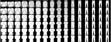
How properly did that work? Let’s see the sorts of garments generated after 50 epochs.

Additionally, how disentangled (or not) are the completely different courses in latent area?

And now watch completely different garments morph into each other.

How good are these representations? That is exhausting to say when there’s nothing to check with.

So let’s dive into MMD-VAE and see the way it does on the identical dataset.

MMD-VAE

MMD-VAE guarantees to generate extra informative latent options, so we might hope to see completely different habits particularly within the clustering and morphing plots.

Information setup is identical, and there are solely very slight variations within the mannequin. Please take a look at the entire code for this instance, mmd_vae.R, as right here we’ll simply spotlight the variations.

Variations within the mannequin(s)

There are three variations as regards mannequin structure.

One, the encoder doesn’t should return the variance, so there isn’t any want for tf$cut up. The encoder’s name methodology now simply is

perform (x, masks = NULL) {
  x %>%
    self$conv1() %>%
    self$conv2() %>%
    self$flatten() %>%
    self$dense() 
}

Between the encoder and the decoder, we don’t want the sampling step anymore, so there isn’t any reparameterization.
And since we gained’t use tf$nn$sigmoid_cross_entropy_with_logits to compute the loss, we let the decoder apply the sigmoid within the final deconvolution layer:

self$deconv3 <- layer_conv_2d_transpose(
  filters = 1,
  kernel_size = 3,
  strides = 1,
  padding = "similar",
  activation = "sigmoid"
)

Loss calculations

Now, as anticipated, the large novelty is within the loss perform.

The loss, most imply discrepancy (MMD), relies on the concept two distributions are similar if and provided that all moments are similar.
Concretely, MMD is estimated utilizing a kernel, such because the Gaussian kernel

[k(z,z’)=frac{e^}{2sigma^2}]

to evaluate similarity between distributions.

The concept then is that if two distributions are similar, the common similarity between samples from every distribution needs to be similar to the common similarity between blended samples from each distributions:

[MMD(p(z)||q(z))=E_{p(z),p(z’)}[k(z,z’)]+E_{q(z),q(z’)}[k(z,z’)]−2E_{p(z),q(z’)}[k(z,z’)]]
The next code is a direct port of the writer’s original TensorFlow code:

compute_kernel <- perform(x, y) {
  x_size <- k_shape(x)[1]
  y_size <- k_shape(y)[1]
  dim <- k_shape(x)[2]
  tiled_x <- k_tile(
    k_reshape(x, k_stack(list(x_size, 1, dim))),
    k_stack(list(1, y_size, 1))
  )
  tiled_y <- k_tile(
    k_reshape(y, k_stack(list(1, y_size, dim))),
    k_stack(list(x_size, 1, 1))
  )
  k_exp(-k_mean(k_square(tiled_x - tiled_y), axis = 3) /
          k_cast(dim, tf$float64))
}

compute_mmd <- perform(x, y, sigma_sqr = 1) {
  x_kernel <- compute_kernel(x, x)
  y_kernel <- compute_kernel(y, y)
  xy_kernel <- compute_kernel(x, y)
  k_mean(x_kernel) + k_mean(y_kernel) - 2 * k_mean(xy_kernel)
}

Coaching loop

The coaching loop differs from the usual VAE instance solely within the loss calculations.
Listed below are the respective strains:

 with(tf$GradientTape(persistent = TRUE) %as% tape, {
      
      imply <- encoder(x)
      preds <- decoder(imply)
      
      true_samples <- k_random_normal(
        form = c(batch_size, latent_dim),
        dtype = tf$float64
      )
      loss_mmd <- compute_mmd(true_samples, imply)
      loss_nll <- k_mean(k_square(x - preds))
      loss <- loss_nll + loss_mmd
      
    })

So we merely compute MMD loss in addition to reconstruction loss, and add them up. No sampling is concerned on this model.
In fact, we’re curious to see how properly that labored!

Outcomes

Once more, let’s have a look at some generated garments first. It looks as if edges are a lot sharper right here.

The clusters too look extra properly unfold out within the two dimensions. And, they’re centered at (0,0), as we might have hoped for.

Lastly, let’s see garments morph into each other. Right here, the graceful, steady evolutions are spectacular!
Additionally, almost all area is crammed with significant objects, which hasn’t been the case above.

MNIST

For curiosity’s sake, we generated the identical sorts of plots after coaching on authentic MNIST.
Right here, there are hardly any variations seen in generated random digits after 50 epochs of coaching.

Additionally the variations in clustering aren’t that huge.

However right here too, the morphing seems to be way more natural with MMD-VAE.

Conclusion

To us, this demonstrates impressively what huge a distinction the price perform could make when working with VAEs.
One other part open to experimentation often is the prior used for the latent area – see this talk for an outline of different priors and the “Variational Combination of Posteriors” paper (Tomczak and Welling 2017) for a well-liked current strategy.

For each value capabilities and priors, we anticipate efficient variations to grow to be means larger nonetheless after we go away the managed atmosphere of (Trend) MNIST and work with real-world datasets.