You certain? A Bayesian strategy to acquiring uncertainty estimates from neural networks
If there have been a set of survival guidelines for information scientists, amongst them must be this: At all times report uncertainty estimates together with your predictions. Nonetheless, right here we’re, working with neural networks, and in contrast to lm, a Keras mannequin doesn’t conveniently output one thing like a commonplace error for the weights.
We would strive to consider rolling your personal uncertainty measure – for instance, averaging predictions from networks educated from completely different random weight initializations, for various numbers of epochs, or on completely different subsets of the info. However we’d nonetheless be apprehensive that our technique is kind of a bit, properly … advert hoc.
On this publish, we’ll see a each sensible in addition to theoretically grounded strategy to acquiring uncertainty estimates from neural networks. First, nonetheless, let’s rapidly discuss why uncertainty is that essential – over and above its potential to avoid wasting an information scientist’s job.
Why uncertainty?
In a society the place automated algorithms are – and might be – entrusted with increasingly more life-critical duties, one reply instantly jumps to thoughts: If the algorithm accurately quantifies its uncertainty, we might have human specialists examine the extra unsure predictions and probably revise them.
This can solely work if the community’s self-indicated uncertainty actually is indicative of a better likelihood of misclassification. Leibig et al.(Leibig et al. 2017) used a predecessor of the strategy described under to evaluate neural community uncertainty in detecting diabetic retinopathy. They discovered that certainly, the distributions of uncertainty had been completely different relying on whether or not the reply was appropriate or not:

Along with quantifying uncertainty, it could actually make sense to qualify it. Within the Bayesian deep studying literature, a distinction is usually made between epistemic uncertainty and aleatoric uncertainty (Kendall and Gal 2017).
Epistemic uncertainty refers to imperfections within the mannequin – within the restrict of infinite information, this sort of uncertainty needs to be reducible to 0. Aleatoric uncertainty is because of information sampling and measurement processes and doesn’t rely on the dimensions of the dataset.
Say we practice a mannequin for object detection. With extra information, the mannequin ought to change into extra certain about what makes a unicycle completely different from a mountainbike. Nonetheless, let’s assume all that’s seen of the mountainbike is the entrance wheel, the fork and the top tube. Then it doesn’t look so completely different from a unicycle any extra!
What could be the results if we may distinguish each forms of uncertainty? If epistemic uncertainty is excessive, we are able to attempt to get extra coaching information. The remaining aleatoric uncertainty ought to then hold us cautioned to consider security margins in our utility.
Most likely no additional justifications are required of why we’d wish to assess mannequin uncertainty – however how can we do that?
Uncertainty estimates by means of Bayesian deep studying
In a Bayesian world, in precept, uncertainty is at no cost as we don’t simply get level estimates (the utmost aposteriori) however the full posterior distribution. Strictly talking, in Bayesian deep studying, priors needs to be put over the weights, and the posterior be decided in keeping with Bayes’ rule.
To the deep studying practitioner, this sounds fairly arduous – and the way do you do it utilizing Keras?
In 2016 although, Gal and Ghahramani (Yarin Gal and Ghahramani 2016) confirmed that when viewing a neural community as an approximation to a Gaussian course of, uncertainty estimates will be obtained in a theoretically grounded but very sensible means: by coaching a community with dropout after which, utilizing dropout at take a look at time too. At take a look at time, dropout lets us extract Monte Carlo samples from the posterior, which may then be used to approximate the true posterior distribution.
That is already excellent news, nevertheless it leaves one query open: How can we select an applicable dropout fee? The reply is: let the community study it.
Studying dropout and uncertainty
In a number of 2017 papers (Y. Gal, Hron, and Kendall 2017),(Kendall and Gal 2017), Gal and his coworkers demonstrated how a community will be educated to dynamically adapt the dropout fee so it’s sufficient for the quantity and traits of the info given.
Moreover the predictive imply of the goal variable, it could actually moreover be made to study the variance.
This implies we are able to calculate each forms of uncertainty, epistemic and aleatoric, independently, which is beneficial within the mild of their completely different implications. We then add them as much as receive the general predictive uncertainty.
Let’s make this concrete and see how we are able to implement and take a look at the supposed habits on simulated information.
Within the implementation, there are three issues warranting our particular consideration:
- The wrapper class used so as to add learnable-dropout habits to a Keras layer;
- The loss perform designed to attenuate aleatoric uncertainty; and
- The methods we are able to receive each uncertainties at take a look at time.
Let’s begin with the wrapper.
A wrapper for studying dropout
On this instance, we’ll limit ourselves to studying dropout for dense layers. Technically, we’ll add a weight and a loss to each dense layer we wish to use dropout with. This implies we’ll create a custom wrapper class that has entry to the underlying layer and might modify it.
The logic carried out within the wrapper is derived mathematically within the Concrete Dropout paper (Y. Gal, Hron, and Kendall 2017). The under code is a port to R of the Python Keras model discovered within the paper’s companion github repo.
So first, right here is the wrapper class – we’ll see methods to use it in only a second:
library(keras)

# R6 wrapper class, a subclass of KerasWrapper
ConcreteDropout <- R6::R6Class("ConcreteDropout",

  inherit = KerasWrapper,

  public = list(
    weight_regularizer = NULL,
    dropout_regularizer = NULL,
    init_min = NULL,
    init_max = NULL,
    is_mc_dropout = NULL,
    supports_masking = TRUE,
    p_logit = NULL,
    p = NULL,

    initialize = perform(weight_regularizer,
                          dropout_regularizer,
                          init_min,
                          init_max,
                          is_mc_dropout) {
      self$weight_regularizer <- weight_regularizer
      self$dropout_regularizer <- dropout_regularizer
      self$is_mc_dropout <- is_mc_dropout
      self$init_min <- k_log(init_min) - k_log(1 - init_min)
      self$init_max <- k_log(init_max) - k_log(1 - init_max)
    },

    construct = perform(input_shape) {
      tremendous$construct(input_shape)

      self$p_logit <- tremendous$add_weight(
        title = "p_logit",
        form = form(1),
        initializer = initializer_random_uniform(self$init_min, self$init_max),
        trainable = TRUE
      )

      self$p <- k_sigmoid(self$p_logit)

      input_dim <- input_shape[[2]]

      weight <- personal$py_wrapper$layer$kernel

      kernel_regularizer <- self$weight_regularizer *
                            k_sum(k_square(weight)) /
                            (1 - self$p)

      dropout_regularizer <- self$p * k_log(self$p)
      dropout_regularizer <- dropout_regularizer +
                             (1 - self$p) * k_log(1 - self$p)
      dropout_regularizer <- dropout_regularizer *
                             self$dropout_regularizer *
                             k_cast(input_dim, k_floatx())

      regularizer <- k_sum(kernel_regularizer + dropout_regularizer)
      tremendous$add_loss(regularizer)
    },

    concrete_dropout = perform(x) {
      eps <- k_cast_to_floatx(k_epsilon())
      temp <- 0.1

      unif_noise <- k_random_uniform(form = k_shape(x))

      drop_prob <- k_log(self$p + eps) -
                   k_log(1 - self$p + eps) +
                   k_log(unif_noise + eps) -
                   k_log(1 - unif_noise + eps)
      drop_prob <- k_sigmoid(drop_prob / temp)

      random_tensor <- 1 - drop_prob

      retain_prob <- 1 - self$p
      x <- x * random_tensor
      x <- x / retain_prob
      x
    },

    name = perform(x, masks = NULL, coaching = NULL) {
      if (self$is_mc_dropout) {
        tremendous$name(self$concrete_dropout(x))
      } else {
        k_in_train_phase(
          perform()
            tremendous$name(self$concrete_dropout(x)),
          tremendous$name(x),
          coaching = coaching
        )
      }
    }
  )
)

# perform for instantiating customized wrapper
layer_concrete_dropout <- perform(object,
                                   layer,
                                   weight_regularizer = 1e-6,
                                   dropout_regularizer = 1e-5,
                                   init_min = 0.1,
                                   init_max = 0.1,
                                   is_mc_dropout = TRUE,
                                   title = NULL,
                                   trainable = TRUE) {
  create_wrapper(ConcreteDropout, object, list(
    layer = layer,
    weight_regularizer = weight_regularizer,
    dropout_regularizer = dropout_regularizer,
    init_min = init_min,
    init_max = init_max,
    is_mc_dropout = is_mc_dropout,
    title = title,
    trainable = trainable
  ))
}
The wrapper instantiator has default arguments, however two of them needs to be tailored to the info: weight_regularizer and dropout_regularizer. Following the authors’ suggestions, they need to be set as follows.
First, select a price for hyperparameter (l). On this view of a neural community as an approximation to a Gaussian course of, (l) is the prior length-scale, our a priori assumption in regards to the frequency traits of the info. Right here, we comply with Gal’s demo in setting l := 1e-4. Then the preliminary values for weight_regularizer and dropout_regularizer are derived from the length-scale and the pattern dimension.
# pattern dimension (coaching information)
n_train <- 1000
# pattern dimension (validation information)
n_val <- 1000
# prior length-scale
l <- 1e-4
# preliminary worth for weight regularizer
wd <- l^2/n_train
# preliminary worth for dropout regularizer
dd <- 2/n_train
Now let’s see methods to use the wrapper in a mannequin.
Dropout mannequin
In our demonstration, we’ll have a mannequin with three hidden dense layers, every of which may have its dropout fee calculated by a devoted wrapper.
# we use one-dimensional enter information right here, however this is not a necessity
input_dim <- 1
# this too might be > 1 if we needed
output_dim <- 1
hidden_dim <- 1024

enter <- layer_input(form = input_dim)

output <- enter %>% layer_concrete_dropout(
  layer = layer_dense(models = hidden_dim, activation = "relu"),
  weight_regularizer = wd,
  dropout_regularizer = dd
  ) %>% layer_concrete_dropout(
  layer = layer_dense(models = hidden_dim, activation = "relu"),
  weight_regularizer = wd,
  dropout_regularizer = dd
  ) %>% layer_concrete_dropout(
  layer = layer_dense(models = hidden_dim, activation = "relu"),
  weight_regularizer = wd,
  dropout_regularizer = dd
)
Now, mannequin output is attention-grabbing: We’ve got the mannequin yielding not simply the predictive (conditional) imply, but in addition the predictive variance ((tau^{-1}) in Gaussian course of parlance):
imply <- output %>% layer_concrete_dropout(
  layer = layer_dense(models = output_dim),
  weight_regularizer = wd,
  dropout_regularizer = dd
)

log_var <- output %>% layer_concrete_dropout(
  layer_dense(models = output_dim),
  weight_regularizer = wd,
  dropout_regularizer = dd
)

output <- layer_concatenate(list(imply, log_var))

mannequin <- keras_model(enter, output)
The numerous factor right here is that we study completely different variances for various information factors. We thus hope to have the ability to account for heteroscedasticity (completely different levels of variability) within the information.
Heteroscedastic loss
Accordingly, as an alternative of imply squared error we use a value perform that doesn’t deal with all estimates alike(Kendall and Gal 2017):
[frac{1}{N} sum_i{frac{1}{2 hat{sigma}^2_i} (mathbf{y}_i – mathbf{hat{y}}_i)^2 + frac{1}{2} log hat{sigma}^2_i}]
Along with the compulsory goal vs. prediction verify, this value perform accommodates two regularization phrases:
- First, (frac{1}{2 hat{sigma}^2_i}) downweights the high-uncertainty predictions within the loss perform. Put plainly: The mannequin is inspired to point excessive uncertainty when its predictions are false.
- Second, (frac{1}{2} log hat{sigma}^2_i) makes certain the community doesn’t merely point out excessive uncertainty all over the place.
This logic maps on to the code (besides that as regular, we’re calculating with the log of the variance, for causes of numerical stability):
heteroscedastic_loss <- perform(y_true, y_pred) {
    imply <- y_pred[, 1:output_dim]
    log_var <- y_pred[, (output_dim + 1):(output_dim * 2)]
    precision <- k_exp(-log_var)
    k_sum(precision * (y_true - imply) ^ 2 + log_var, axis = 2)
  }
Coaching on simulated information
Now we generate some take a look at information and practice the mannequin.
gen_data_1d <- perform(n) {
  sigma <- 1
  X <- matrix(rnorm(n))
  w <- 2
  b <- 8
  Y <- matrix(X %*% w + b + sigma * rnorm(n))
  list(X, Y)
}

c(X, Y) %<-% gen_data_1d(n_train + n_val)

c(X_train, Y_train) %<-% list(X[1:n_train], Y[1:n_train])
c(X_val, Y_val) %<-% list(X[(n_train + 1):(n_train + n_val)],
                          Y[(n_train + 1):(n_train + n_val)])

mannequin %>% compile(
  optimizer = "adam",
  loss = heteroscedastic_loss,
  metrics = c(custom_metric("heteroscedastic_loss", heteroscedastic_loss))
)

historical past <- mannequin %>% match(
  X_train,
  Y_train,
  epochs = 30,
  batch_size = 10
)
With coaching completed, we flip to the validation set to acquire estimates on unseen information – together with these uncertainty measures that is all about!
Acquire uncertainty estimates through Monte Carlo sampling
As typically in a Bayesian setup, we assemble the posterior (and thus, the posterior predictive) through Monte Carlo sampling.
Not like in conventional use of dropout, there is no such thing as a change in habits between coaching and take a look at phases: Dropout stays “on.”
So now we get an ensemble of mannequin predictions on the validation set:
Bear in mind, our mannequin predicts the imply in addition to the variance. We’ll use the previous for calculating epistemic uncertainty, whereas aleatoric uncertainty is obtained from the latter.
First, we decide the predictive imply as a mean of the MC samples’ imply output:
# the means are within the first output column
means <- MC_samples[, , 1:output_dim]
# common over the MC samples
predictive_mean <- apply(means, 2, imply)
To calculate epistemic uncertainty, we once more use the imply output, however this time we’re within the variance of the MC samples:
epistemic_uncertainty <- apply(means, 2, var) Then aleatoric uncertainty is the typical over the MC samples of the variance output..
Notice how this process offers us uncertainty estimates individually for each prediction. How do they appear?
df <- data.frame(
x = X_val,
y_pred = predictive_mean,
e_u_lower = predictive_mean - sqrt(epistemic_uncertainty),
e_u_upper = predictive_mean + sqrt(epistemic_uncertainty),
a_u_lower = predictive_mean - sqrt(aleatoric_uncertainty),
a_u_upper = predictive_mean + sqrt(aleatoric_uncertainty),
u_overall_lower = predictive_mean -
sqrt(epistemic_uncertainty) -
sqrt(aleatoric_uncertainty),
u_overall_upper = predictive_mean +
sqrt(epistemic_uncertainty) +
sqrt(aleatoric_uncertainty)
)Right here, first, is epistemic uncertainty, with shaded bands indicating one commonplace deviation above resp. under the expected imply:
ggplot(df, aes(x, y_pred)) +
geom_point() +
geom_ribbon(aes(ymin = e_u_lower, ymax = e_u_upper), alpha = 0.3)
That is attention-grabbing. The coaching information (in addition to the validation information) had been generated from a regular regular distribution, so the mannequin has encountered many extra examples near the imply than exterior two, and even three, commonplace deviations. So it accurately tells us that in these extra unique areas, it feels fairly not sure about its predictions.
That is precisely the habits we wish: Danger in mechanically making use of machine studying strategies arises as a consequence of unanticipated variations between the coaching and take a look at (actual world) distributions. If the mannequin had been to inform us “ehm, not likely seen something like that earlier than, don’t actually know what to do” that’d be an enormously invaluable end result.
So whereas epistemic uncertainty has the algorithm reflecting on its mannequin of the world – probably admitting its shortcomings – aleatoric uncertainty, by definition, is irreducible. In fact, that doesn’t make it any much less invaluable – we’d know we all the time need to consider a security margin. So how does it look right here?

Certainly, the extent of uncertainty doesn’t rely on the quantity of information seen at coaching time.
Lastly, we add up each sorts to acquire the general uncertainty when making predictions.

Now let’s do that technique on a real-world dataset.
Mixed cycle energy plant electrical power output estimation
This dataset is on the market from the UCI Machine Learning Repository. We explicitly selected a regression activity with steady variables completely, to make for a easy transition from the simulated information.
Within the dataset suppliers’ own words
The dataset accommodates 9568 information factors collected from a Mixed Cycle Energy Plant over 6 years (2006-2011), when the ability plant was set to work with full load. Options include hourly common ambient variables Temperature (T), Ambient Stress (AP), Relative Humidity (RH) and Exhaust Vacuum (V) to foretell the web hourly electrical power output (EP) of the plant.
A mixed cycle energy plant (CCPP) consists of fuel generators (GT), steam generators (ST) and warmth restoration steam mills. In a CCPP, the electrical energy is generated by fuel and steam generators, that are mixed in a single cycle, and is transferred from one turbine to a different. Whereas the Vacuum is collected from and has impact on the Steam Turbine, the opposite three of the ambient variables impact the GT efficiency.
We thus have 4 predictors and one goal variable. We’ll practice 5 fashions: 4 single-variable regressions and one making use of all 4 predictors. It most likely goes with out saying that our purpose right here is to examine uncertainty info, to not fine-tune the mannequin.
Setup
Let’s rapidly examine these 5 variables. Right here PE is power output, the goal variable.

We scale and divide up the info
and prepare for coaching a couple of fashions.
n <- nrow(X_train)
n_epochs <- 100
batch_size <- 100
output_dim <- 1
num_MC_samples <- 20
l <- 1e-4
wd <- l^2/n
dd <- 2/n
get_model <- perform(input_dim, hidden_dim) {
enter <- layer_input(form = input_dim)
output <-
enter %>% layer_concrete_dropout(
layer = layer_dense(models = hidden_dim, activation = "relu"),
weight_regularizer = wd,
dropout_regularizer = dd
) %>% layer_concrete_dropout(
layer = layer_dense(models = hidden_dim, activation = "relu"),
weight_regularizer = wd,
dropout_regularizer = dd
) %>% layer_concrete_dropout(
layer = layer_dense(models = hidden_dim, activation = "relu"),
weight_regularizer = wd,
dropout_regularizer = dd
)
imply <-
output %>% layer_concrete_dropout(
layer = layer_dense(models = output_dim),
weight_regularizer = wd,
dropout_regularizer = dd
)
log_var <-
output %>% layer_concrete_dropout(
layer_dense(models = output_dim),
weight_regularizer = wd,
dropout_regularizer = dd
)
output <- layer_concatenate(list(imply, log_var))
mannequin <- keras_model(enter, output)
heteroscedastic_loss <- perform(y_true, y_pred) {
imply <- y_pred[, 1:output_dim]
log_var <- y_pred[, (output_dim + 1):(output_dim * 2)]
precision <- k_exp(-log_var)
k_sum(precision * (y_true - imply) ^ 2 + log_var, axis = 2)
}
mannequin %>% compile(optimizer = "adam",
loss = heteroscedastic_loss,
metrics = c("mse"))
mannequin
}We’ll practice every of the 5 fashions with a hidden_dim of 64.
We then receive 20 Monte Carlo pattern from the posterior predictive distribution and calculate the uncertainties as earlier than.
Right here we present the code for the primary predictor, “AT.” It’s related for all different instances.
mannequin <- get_model(1, 64)
hist <- mannequin %>% match(
X_train[ ,1],
y_train,
validation_data = list(X_val[ , 1], y_val),
epochs = n_epochs,
batch_size = batch_size
)
MC_samples <- array(0, dim = c(num_MC_samples, nrow(X_val), 2 * output_dim))
for (ok in 1:num_MC_samples) {
MC_samples[k, ,] <- (mannequin %>% predict(X_val[ ,1]))
}
means <- MC_samples[, , 1:output_dim]
predictive_mean <- apply(means, 2, imply)
epistemic_uncertainty <- apply(means, 2, var)
logvar <- MC_samples[, , (output_dim + 1):(output_dim * 2)]
aleatoric_uncertainty <- exp(colMeans(logvar))
preds <- data.frame(
x1 = X_val[, 1],
y_true = y_val,
y_pred = predictive_mean,
e_u_lower = predictive_mean - sqrt(epistemic_uncertainty),
e_u_upper = predictive_mean + sqrt(epistemic_uncertainty),
a_u_lower = predictive_mean - sqrt(aleatoric_uncertainty),
a_u_upper = predictive_mean + sqrt(aleatoric_uncertainty),
u_overall_lower = predictive_mean -
sqrt(epistemic_uncertainty) -
sqrt(aleatoric_uncertainty),
u_overall_upper = predictive_mean +
sqrt(epistemic_uncertainty) +
sqrt(aleatoric_uncertainty)
)Consequence
Now let’s see the uncertainty estimates for all 5 fashions!
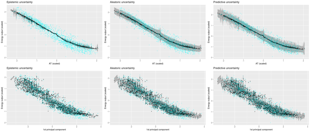
First, the single-predictor setup. Floor reality values are displayed in cyan, posterior predictive estimates are black, and the gray bands prolong up resp. down by the sq. root of the calculated uncertainties.
We’re beginning with ambient temperature, a low-variance predictor.
We’re shocked how assured the mannequin is that it’s gotten the method logic appropriate, however excessive aleatoric uncertainty makes up for this (kind of).

Now trying on the different predictors, the place variance is far greater within the floor reality, it does get a bit tough to really feel comfy with the mannequin’s confidence. Aleatoric uncertainty is excessive, however not excessive sufficient to seize the true variability within the information. And we certaintly would hope for greater epistemic uncertainty, particularly in locations the place the mannequin introduces arbitrary-looking deviations from linearity.


Now let’s see uncertainty output after we use all 4 predictors. We see that now, the Monte Carlo estimates fluctuate much more, and accordingly, epistemic uncertainty is quite a bit greater. Aleatoric uncertainty, then again, bought quite a bit decrease. General, predictive uncertainty captures the vary of floor reality values fairly properly.

Conclusion
We’ve launched a way to acquire theoretically grounded uncertainty estimates from neural networks.
We discover the strategy intuitively engaging for a number of causes: For one, the separation of various kinds of uncertainty is convincing and virtually related. Second, uncertainty is dependent upon the quantity of information seen within the respective ranges. That is particularly related when pondering of variations between coaching and test-time distributions.
Third, the concept of getting the community “change into conscious of its personal uncertainty” is seductive.
In observe although, there are open questions as to methods to apply the strategy. From our real-world take a look at above, we instantly ask: Why is the mannequin so assured when the bottom reality information has excessive variance? And, pondering experimentally: How would that adjust with completely different information sizes (rows), dimensionality (columns), and hyperparameter settings (together with neural community hyperparameters like capability, variety of epochs educated, and activation capabilities, but in addition the Gaussian course of prior length-scale (tau))?
For sensible use, extra experimentation with completely different datasets and hyperparameter settings is actually warranted.
One other path to comply with up is utility to duties in picture recognition, akin to semantic segmentation.
Right here we’d be inquisitive about not simply quantifying, but in addition localizing uncertainty, to see which visible points of a scene (occlusion, illumination, unusual shapes) make objects onerous to determine.


