Discrete Illustration Studying with VQ-VAE and TensorFlow Likelihood
About two weeks in the past, we introduced TensorFlow Probability (TFP), displaying how you can create and pattern from distributions and put them to make use of in a Variational Autoencoder (VAE) that learns its prior. At present, we transfer on to a unique specimen within the VAE mannequin zoo: the Vector Quantised Variational Autoencoder (VQ-VAE) described in Neural Discrete Illustration Studying (Oord, Vinyals, and Kavukcuoglu 2017). This mannequin differs from most VAEs in that its approximate posterior shouldn’t be steady, however discrete – therefore the “quantised” within the article’s title. We’ll rapidly have a look at what this implies, after which dive immediately into the code, combining Keras layers, keen execution, and TFP.
Many phenomena are greatest considered, and modeled, as discrete. This holds for phonemes and lexemes in language, higher-level buildings in pictures (suppose objects as a substitute of pixels),and duties that necessitate reasoning and planning.
The latent code utilized in most VAEs, nevertheless, is steady – normally it’s a multivariate Gaussian. Steady-space VAEs have been discovered very profitable in reconstructing their enter, however typically they endure from one thing referred to as posterior collapse: The decoder is so highly effective that it could create practical output given simply any enter. This implies there isn’t any incentive to be taught an expressive latent area.
In VQ-VAE, nevertheless, every enter pattern will get mapped deterministically to certainly one of a set of embedding vectors. Collectively, these embedding vectors represent the prior for the latent area.
As such, an embedding vector comprises much more info than a imply and a variance, and thus, is way tougher to disregard by the decoder.
The query then is: The place is that magical hat, for us to tug out significant embeddings?
From the above conceptual description, we now have two inquiries to reply. First, by what mechanism will we assign enter samples (that went via the encoder) to applicable embedding vectors?
And second: How can we be taught embedding vectors that truly are helpful representations – that when fed to a decoder, will lead to entities perceived as belonging to the identical species?
As regards task, a tensor emitted from the encoder is just mapped to its nearest neighbor in embedding area, utilizing Euclidean distance. The embedding vectors are then up to date utilizing exponential shifting averages. As we’ll see quickly, which means that they’re really not being discovered utilizing gradient descent – a characteristic value stating as we don’t come throughout it daily in deep studying.
Concretely, how then ought to the loss operate and coaching course of look? This may most likely best be seen in code.
The whole code for this instance, together with utilities for mannequin saving and picture visualization, is available on github as a part of the Keras examples. Order of presentation right here might differ from precise execution order for expository functions, so please to truly run the code think about making use of the instance on github.
As in all our prior posts on VAEs, we use keen execution, which presupposes the TensorFlow implementation of Keras.
As in our earlier put up on doing VAE with TFP, we’ll use Kuzushiji-MNIST(Clanuwat et al. 2018) as enter.
Now’s the time to have a look at what we ended up generating that time and place your guess: How will that examine towards the discrete latent area of VQ-VAE?
np <- import("numpy")

kuzushiji <- np$load("kmnist-train-imgs.npz")
kuzushiji <- kuzushiji$get("arr_0")

train_images <- kuzushiji %>%
  k_expand_dims() %>%
  k_cast(dtype = "float32")

train_images <- train_images %>% `/`(255)

buffer_size <- 60000
batch_size <- 64
num_examples_to_generate <- batch_size

batches_per_epoch <- buffer_size / batch_size

train_dataset <- tensor_slices_dataset(train_images) %>%
  dataset_shuffle(buffer_size) %>%
  dataset_batch(batch_size, drop_remainder = TRUE)
Hyperparameters
Along with the “normal” hyperparameters now we have in deep studying, the VQ-VAE infrastructure introduces a number of model-specific ones. To start with, the embedding area is of dimensionality variety of embedding vectors instances embedding vector measurement:
# variety of embedding vectors
num_codes <- 64L
# dimensionality of the embedding vectors
code_size <- 16L
The latent area in our instance shall be of measurement one, that’s, now we have a single embedding vector representing the latent code for every enter pattern. This shall be effective for our dataset, nevertheless it must be famous that van den Oord et al. used far higher-dimensional latent areas on e.g. ImageNet and Cifar-10.
Encoder mannequin
The encoder makes use of convolutional layers to extract picture options. Its output is a three-D tensor of form batchsize * 1 * code_size.
activation <- "elu"
# modularizing the code just a bit bit
default_conv <- set_defaults(layer_conv_2d, list(padding = "similar", activation = activation))
base_depth <- 32
encoder_model <- operate(title = NULL,
code_size) {
keras_model_custom(title = title, operate(self) {
self$conv1 <- default_conv(filters = base_depth, kernel_size = 5)
self$conv2 <- default_conv(filters = base_depth, kernel_size = 5, strides = 2)
self$conv3 <- default_conv(filters = 2 * base_depth, kernel_size = 5)
self$conv4 <- default_conv(filters = 2 * base_depth, kernel_size = 5, strides = 2)
self$conv5 <- default_conv(filters = 4 * latent_size, kernel_size = 7, padding = "legitimate")
self$flatten <- layer_flatten()
self$dense <- layer_dense(models = latent_size * code_size)
self$reshape <- layer_reshape(target_shape = c(latent_size, code_size))
operate (x, masks = NULL) {
x %>%
# output form: 7 28 28 32
self$conv1() %>%
# output form: 7 14 14 32
self$conv2() %>%
# output form: 7 14 14 64
self$conv3() %>%
# output form: 7 7 7 64
self$conv4() %>%
# output form: 7 1 1 4
self$conv5() %>%
# output form: 7 4
self$flatten() %>%
# output form: 7 16
self$dense() %>%
# output form: 7 1 16
self$reshape()
}
})
}As at all times, let’s make use of the truth that we’re utilizing keen execution, and see a number of instance outputs.
iter <- make_iterator_one_shot(train_dataset)
batch <-  iterator_get_next(iter)

encoder <- encoder_model(code_size = code_size)
encoded  <- encoder(batch)
encoded
tf.Tensor(
[[[ 0.00516277 -0.00746826 0.0268365 ... -0.012577 -0.07752544
-0.02947626]]
...
[[-0.04757921 -0.07282603 -0.06814402 ... -0.10861694 -0.01237121
0.11455103]]], form=(64, 1, 16), dtype=float32)Now, every of those 16d vectors must be mapped to the embedding vector it’s closest to. This mapping is taken care of by one other mannequin: vector_quantizer.
Vector quantizer mannequin
That is how we are going to instantiate the vector quantizer:
vector_quantizer <- vector_quantizer_model(num_codes = num_codes, code_size = code_size)This mannequin serves two functions: First, it acts as a retailer for the embedding vectors. Second, it matches encoder output to out there embeddings.
Right here, the present state of embeddings is saved in codebook. ema_means and ema_count are for bookkeeping functions solely (notice how they’re set to be non-trainable). We’ll see them in use shortly.
vector_quantizer_model <- operate(title = NULL, num_codes, code_size) {

    keras_model_custom(title = title, operate(self) {

      self$num_codes <- num_codes
      self$code_size <- code_size
      self$codebook <- tf$get_variable(
        "codebook",
        form = c(num_codes, code_size),
        dtype = tf$float32
        )
      self$ema_count <- tf$get_variable(
        title = "ema_count", form = c(num_codes),
        initializer = tf$constant_initializer(0),
        trainable = FALSE
        )
      self$ema_means = tf$get_variable(
        title = "ema_means",
        initializer = self$codebook$initialized_value(),
        trainable = FALSE
        )

      operate (x, masks = NULL) {

        # to be crammed in shortly ...

      }
    })
}
Along with the precise embeddings, in its name technique vector_quantizer holds the task logic.
First, we compute the Euclidean distance of every encoding to the vectors within the codebook (tf$norm).
We assign every encoding to the closest as by that distance embedding (tf$argmin) and one-hot-encode the assignments (tf$one_hot). Lastly, we isolate the corresponding vector by masking out all others and summing up what’s left over (multiplication adopted by tf$reduce_sum).
Relating to the axis argument used with many TensorFlow features, please consider that in distinction to their k_* siblings, uncooked TensorFlow (tf$*) features anticipate axis numbering to be 0-based. We even have so as to add the L’s after the numbers to evolve to TensorFlow’s datatype necessities.
vector_quantizer_model <- operate(title = NULL, num_codes, code_size) {

    keras_model_custom(title = title, operate(self) {

      # right here now we have the above occasion fields

      operate (x, masks = NULL) {

        # form: bs * 1 * num_codes
         distances <- tf$norm(
          tf$expand_dims(x, axis = 2L) -
            tf$reshape(self$codebook,
                       c(1L, 1L, self$num_codes, self$code_size)),
                       axis = 3L
        )

        # bs * 1
        assignments <- tf$argmin(distances, axis = 2L)

        # bs * 1 * num_codes
        one_hot_assignments <- tf$one_hot(assignments, depth = self$num_codes)

        # bs * 1 * code_size
        nearest_codebook_entries <- tf$reduce_sum(
          tf$expand_dims(
            one_hot_assignments, -1L) *
            tf$reshape(self$codebook, c(1L, 1L, self$num_codes, self$code_size)),
                       axis = 2L
                       )
        list(nearest_codebook_entries, one_hot_assignments)
      }
    })
  }
Now that we’ve seen how the codes are saved, let’s add performance for updating them.
As we mentioned above, they don’t seem to be discovered by way of gradient descent. As an alternative, they’re exponential shifting averages, frequently up to date by no matter new “class member” they get assigned.
So here’s a operate update_ema that can maintain this.
update_ema makes use of TensorFlow moving_averages to
- first, maintain monitor of the variety of at present assigned samples per code (
updated_ema_count), and - second, compute and assign the present exponential shifting common (
updated_ema_means).
moving_averages <- tf$python$coaching$moving_averages

# decay to make use of in computing exponential shifting common
decay <- 0.99

update_ema <- operate(
  vector_quantizer,
  one_hot_assignments,
  codes,
  decay) {

  updated_ema_count <- moving_averages$assign_moving_average(
    vector_quantizer$ema_count,
    tf$reduce_sum(one_hot_assignments, axis = c(0L, 1L)),
    decay,
    zero_debias = FALSE
  )

  updated_ema_means <- moving_averages$assign_moving_average(
    vector_quantizer$ema_means,
    # selects all assigned values (masking out the others) and sums them up over the batch
    # (shall be divided by depend later, so we get a median)
    tf$reduce_sum(
      tf$expand_dims(codes, 2L) *
        tf$expand_dims(one_hot_assignments, 3L), axis = c(0L, 1L)),
    decay,
    zero_debias = FALSE
  )

  updated_ema_count <- updated_ema_count + 1e-5
  updated_ema_means <-  updated_ema_means / tf$expand_dims(updated_ema_count, axis = -1L)

  tf$assign(vector_quantizer$codebook, updated_ema_means)
}
Earlier than we have a look at the coaching loop, let’s rapidly full the scene including within the final actor, the decoder.
Decoder mannequin
The decoder is fairly normal, performing a collection of deconvolutions and at last, returning a chance for every picture pixel.
default_deconv <- set_defaults(
  layer_conv_2d_transpose,
  list(padding = "similar", activation = activation)
)

decoder_model <- operate(title = NULL,
                          input_size,
                          output_shape) {

  keras_model_custom(title = title, operate(self) {

    self$reshape1 <- layer_reshape(target_shape = c(1, 1, input_size))
    self$deconv1 <-
      default_deconv(
        filters = 2 * base_depth,
        kernel_size = 7,
        padding = "legitimate"
      )
    self$deconv2 <-
      default_deconv(filters = 2 * base_depth, kernel_size = 5)
    self$deconv3 <-
      default_deconv(
        filters = 2 * base_depth,
        kernel_size = 5,
        strides = 2
      )
    self$deconv4 <-
      default_deconv(filters = base_depth, kernel_size = 5)
    self$deconv5 <-
      default_deconv(filters = base_depth,
                     kernel_size = 5,
                     strides = 2)
    self$deconv6 <-
      default_deconv(filters = base_depth, kernel_size = 5)
    self$conv1 <-
      default_conv(filters = output_shape[3],
                   kernel_size = 5,
                   activation = "linear")

    operate (x, masks = NULL) {

      x <- x %>%
        # output form:  7 1 1 16
        self$reshape1() %>%
        # output form:  7 7 7 64
        self$deconv1() %>%
        # output form:  7 7 7 64
        self$deconv2() %>%
        # output form:  7 14 14 64
        self$deconv3() %>%
        # output form:  7 14 14 32
        self$deconv4() %>%
        # output form:  7 28 28 32
        self$deconv5() %>%
        # output form:  7 28 28 32
        self$deconv6() %>%
        # output form:  7 28 28 1
        self$conv1()

      tfd$Unbiased(tfd$Bernoulli(logits = x),
                      reinterpreted_batch_ndims = length(output_shape))
    }
  })
}

input_shape <- c(28, 28, 1)
decoder <- decoder_model(input_size = latent_size * code_size,
                         output_shape = input_shape)
Now we’re prepared to coach. One factor we haven’t actually talked about but is the price operate: Given the variations in structure (in comparison with normal VAEs), will the losses nonetheless look as anticipated (the same old add-up of reconstruction loss and KL divergence)?
We’ll see that in a second.
Coaching loop
Right here’s the optimizer we’ll use. Losses shall be calculated inline.
optimizer <- tf$practice$AdamOptimizer(learning_rate = learning_rate)The coaching loop, as normal, is a loop over epochs, the place every iteration is a loop over batches obtained from the dataset.
For every batch, now we have a ahead move, recorded by a gradientTape, primarily based on which we calculate the loss.
The tape will then decide the gradients of all trainable weights all through the mannequin, and the optimizer will use these gradients to replace the weights.
Up to now, all of this conforms to a scheme we’ve oftentimes seen earlier than. One level to notice although: On this similar loop, we additionally name update_ema to recalculate the shifting averages, as these will not be operated on throughout backprop.
Right here is the important performance:
num_epochs <- 20

for (epoch in seq_len(num_epochs)) {

  iter <- make_iterator_one_shot(train_dataset)

  until_out_of_range({

    x <-  iterator_get_next(iter)
    with(tf$GradientTape(persistent = TRUE) %as% tape, {

      # do ahead move
      # calculate losses

    })

    encoder_gradients <- tape$gradient(loss, encoder$variables)
    decoder_gradients <- tape$gradient(loss, decoder$variables)

    optimizer$apply_gradients(purrr::transpose(list(
      encoder_gradients, encoder$variables
    )),
    global_step = tf$practice$get_or_create_global_step())

    optimizer$apply_gradients(purrr::transpose(list(
      decoder_gradients, decoder$variables
    )),
    global_step = tf$practice$get_or_create_global_step())

    update_ema(vector_quantizer,
               one_hot_assignments,
               codes,
               decay)

    # periodically show some generated pictures
    # see code on github
    # visualize_images("kuzushiji", epoch, reconstructed_images, random_images)
  })
}
Now, for the precise motion. Contained in the context of the gradient tape, we first decide which encoded enter pattern will get assigned to which embedding vector.
codes <- encoder(x)
c(nearest_codebook_entries, one_hot_assignments) %<-% vector_quantizer(codes)
Now, for this task operation there isn’t any gradient. As an alternative what we are able to do is move the gradients from decoder enter straight via to encoder output.
Right here tf$stop_gradient exempts nearest_codebook_entries from the chain of gradients, so encoder and decoder are linked by codes:
codes_straight_through <- codes + tf$stop_gradient(nearest_codebook_entries - codes)
decoder_distribution <- decoder(codes_straight_through)
In sum, backprop will maintain the decoder’s in addition to the encoder’s weights, whereas the latent embeddings are up to date utilizing shifting averages, as we’ve seen already.
Now we’re able to deal with the losses. There are three parts:
- First, the reconstruction loss, which is simply the log chance of the particular enter below the distribution discovered by the decoder.
reconstruction_loss <- -tf$reduce_mean(decoder_distribution$log_prob(x))- Second, now we have the dedication loss, outlined because the imply squared deviation of the encoded enter samples from the closest neighbors they’ve been assigned to: We wish the community to “commit” to a concise set of latent codes!
commitment_loss <- tf$reduce_mean(tf$sq.(codes - tf$stop_gradient(nearest_codebook_entries)))- Lastly, now we have the same old KL diverge to a previous. As, a priori, all assignments are equally possible, this element of the loss is fixed and might oftentimes be distributed of. We’re including it right here primarily for illustrative functions.
prior_dist <- tfd$Multinomial(
  total_count = 1,
  logits = tf$zeros(c(latent_size, num_codes))
  )
prior_loss <- -tf$reduce_mean(
  tf$reduce_sum(prior_dist$log_prob(one_hot_assignments), 1L)
  )
Summing up all three parts, we arrive on the general loss:
beta <- 0.25
loss <- reconstruction_loss + beta * commitment_loss + prior_loss
Earlier than we have a look at the outcomes, let’s see what occurs inside gradientTape at a single look:
with(tf$GradientTape(persistent = TRUE) %as% tape, {

  codes <- encoder(x)
  c(nearest_codebook_entries, one_hot_assignments) %<-% vector_quantizer(codes)
  codes_straight_through <- codes + tf$stop_gradient(nearest_codebook_entries - codes)
  decoder_distribution <- decoder(codes_straight_through)

  reconstruction_loss <- -tf$reduce_mean(decoder_distribution$log_prob(x))
  commitment_loss <- tf$reduce_mean(tf$sq.(codes - tf$stop_gradient(nearest_codebook_entries)))
  prior_dist <- tfd$Multinomial(
    total_count = 1,
    logits = tf$zeros(c(latent_size, num_codes))
  )
  prior_loss <- -tf$reduce_mean(tf$reduce_sum(prior_dist$log_prob(one_hot_assignments), 1L))

  loss <- reconstruction_loss + beta * commitment_loss + prior_loss
})
Outcomes
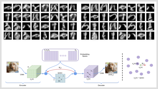
And right here we go. This time, we are able to’t have the 2nd “morphing view” one usually likes to show with VAEs (there simply isn’t any 2nd latent area). As an alternative, the 2 pictures under are (1) letters generated from random enter and (2) reconstructed precise letters, every saved after coaching for 9 epochs.

Two issues bounce to the attention: First, the generated letters are considerably sharper than their continuous-prior counterparts (from the earlier put up). And second, would you’ve been capable of inform the random picture from the reconstruction picture?
At this level, we’ve hopefully satisfied you of the facility and effectiveness of this discrete-latents method.
Nevertheless, you may secretly have hoped we’d apply this to extra advanced information, reminiscent of the weather of speech we talked about within the introduction, or higher-resolution pictures as present in ImageNet.
The reality is that there’s a steady tradeoff between the variety of new and thrilling strategies we are able to present, and the time we are able to spend on iterations to efficiently apply these strategies to advanced datasets. Ultimately it’s you, our readers, who will put these strategies to significant use on related, actual world information.


