Hierarchical partial pooling with tfprobability

Earlier than we bounce into the technicalities: This publish is, in fact, devoted to McElreath who wrote one in every of most intriguing books on Bayesian (or ought to we simply say – scientific?) modeling we’re conscious of. In case you haven’t learn Statistical Rethinking, and are keen on modeling, you may undoubtedly wish to test it out. On this publish, we’re not going to attempt to re-tell the story: Our clear focus will, as a substitute, be an illustration of do MCMC with tfprobability.

Concretely, this publish has two elements. The primary is a fast overview of use tfd_joint_sequential_distribution to assemble a mannequin, after which pattern from it utilizing Hamiltonian Monte Carlo. This half could be consulted for fast code look-up, or as a frugal template of the entire course of.
The second half then walks by way of a multi-level mannequin in additional element, exhibiting extract, post-process and visualize sampling in addition to diagnostic outputs.

Reedfrogs

The info comes with the rethinking bundle.

'information.body':   48 obs. of  5 variables:
 $ density : int  10 10 10 10 10 10 10 10 10 10 ...
 $ pred    : Issue w/ 2 ranges "no","pred": 1 1 1 1 1 1 1 1 2 2 ...
 $ dimension    : Issue w/ 2 ranges "huge","small": 1 1 1 1 2 2 2 2 1 1 ...
 $ surv    : int  9 10 7 10 9 9 10 9 4 9 ...
 $ propsurv: num  0.9 1 0.7 1 0.9 0.9 1 0.9 0.4 0.9 ...

The duty is modeling survivor counts amongst tadpoles, the place tadpoles are held in tanks of various sizes (equivalently, totally different numbers of inhabitants). Every row within the dataset describes one tank, with its preliminary depend of inhabitants (density) and variety of survivors (surv).
Within the technical overview half, we construct a easy unpooled mannequin that describes each tank in isolation. Then, within the detailed walk-through, we’ll see assemble a various intercepts mannequin that permits for data sharing between tanks.

Setting up fashions with tfd_joint_distribution_sequential

tfd_joint_distribution_sequential represents a mannequin as a listing of conditional distributions.
That is best to see on an actual instance, so we’ll bounce proper in, creating an unpooled mannequin of the tadpole information.

That is the how the mannequin specification would look in Stan:

mannequin{
    vector[48] p;
    a ~ regular( 0 , 1.5 );
    for ( i in 1:48 ) {
        p[i] = a[tank[i]];
        p[i] = inv_logit(p[i]);
    }
    S ~ binomial( N , p );
}

And right here is tfd_joint_distribution_sequential:

library(tensorflow)

# ensure you have a minimum of model 0.7 of TensorFlow Chance 
# as of this writing, it's required of set up the grasp department:
# install_tensorflow(model = "nightly")
library(tfprobability)

n_tadpole_tanks <- nrow(d)
n_surviving <- d$surv
n_start <- d$density

m1 <- tfd_joint_distribution_sequential(
  list(
    # regular prior of per-tank logits
    tfd_multivariate_normal_diag(
      loc = rep(0, n_tadpole_tanks),
      scale_identity_multiplier = 1.5),
    # binomial distribution of survival counts
    operate(l)
      tfd_independent(
        tfd_binomial(total_count = n_start, logits = l),
        reinterpreted_batch_ndims = 1
      )
  )
)

The mannequin consists of two distributions: Prior means and variances for the 48 tadpole tanks are specified by tfd_multivariate_normal_diag; then tfd_binomial generates survival counts for every tank.
Observe how the primary distribution is unconditional, whereas the second relies on the primary. Observe too how the second needs to be wrapped in tfd_independent to keep away from incorrect broadcasting. (That is a facet of tfd_joint_distribution_sequential utilization that deserves to be documented extra systematically, which is definitely going to occur. Simply suppose that this performance was added to TFP grasp solely three weeks in the past!)

As an apart, the mannequin specification right here finally ends up shorter than in Stan as tfd_binomial optionally takes logits as parameters.

As with each TFP distribution, you are able to do a fast performance verify by sampling from the mannequin:

# pattern a batch of two values 
# we get samples for each distribution within the mannequin
s <- m1 %>% tfd_sample(2)

[[1]]
Tensor("MultivariateNormalDiag/pattern/affine_linear_operator/ahead/add:0",
form=(2, 48), dtype=float32)

[[2]]
Tensor("IndependentJointDistributionSequential/pattern/Beta/pattern/Reshape:0",
form=(2, 48), dtype=float32)

and computing log possibilities:

# we should always get solely the general log chance of the mannequin
m1 %>% tfd_log_prob(s)

t[[1]]
Tensor("MultivariateNormalDiag/pattern/affine_linear_operator/ahead/add:0",
form=(2, 48), dtype=float32)

[[2]]
Tensor("IndependentJointDistributionSequential/pattern/Beta/pattern/Reshape:0",
form=(2, 48), dtype=float32)

Now, let’s see how we will pattern from this mannequin utilizing Hamiltonian Monte Carlo.

Operating Hamiltonian Monte Carlo in TFP

We outline a Hamiltonian Monte Carlo kernel with dynamic step dimension adaptation primarily based on a desired acceptance chance.

# variety of steps to run burnin
n_burnin <- 500

# optimization goal is the chance of the logits given the info
logprob <- operate(l)
  m1 %>% tfd_log_prob(list(l, n_surviving))

hmc <- mcmc_hamiltonian_monte_carlo(
  target_log_prob_fn = logprob,
  num_leapfrog_steps = 3,
  step_size = 0.1,
) %>%
  mcmc_simple_step_size_adaptation(
    target_accept_prob = 0.8,
    num_adaptation_steps = n_burnin
  )

We then run the sampler, passing in an preliminary state. If we wish to run (n) chains, that state needs to be of size (n), for each parameter within the mannequin (right here we now have only one).

The sampling operate, mcmc_sample_chain, might optionally be handed a trace_fn that tells TFP which sorts of meta data to save lots of. Right here we save acceptance ratios and step sizes.

# variety of steps after burnin
n_steps <- 500
# variety of chains
n_chain <- 4

# get beginning values for the parameters
# their form implicitly determines the variety of chains we'll run
# see current_state parameter handed to mcmc_sample_chain under
c(initial_logits, .) %<-% (m1 %>% tfd_sample(n_chain))

# inform TFP to maintain monitor of acceptance ratio and step dimension
trace_fn <- operate(state, pkr) {
  list(pkr$inner_results$is_accepted,
       pkr$inner_results$accepted_results$step_size)
}

res <- hmc %>% mcmc_sample_chain(
  num_results = n_steps,
  num_burnin_steps = n_burnin,
  current_state = initial_logits,
  trace_fn = trace_fn
)

When sampling is completed, we will entry the samples as res$all_states:

mcmc_trace <- res$all_states
mcmc_trace

Tensor("mcmc_sample_chain/trace_scan/TensorArrayStack/TensorArrayGatherV3:0",
form=(500, 4, 48), dtype=float32)

That is the form of the samples for l, the 48 per-tank logits: 500 samples occasions 4 chains occasions 48 parameters.

From these samples, we will compute efficient pattern dimension and (rhat) (alias mcmc_potential_scale_reduction):

# Tensor("Imply:0", form=(48,), dtype=float32)
ess <- mcmc_effective_sample_size(mcmc_trace) %>% tf$reduce_mean(axis = 0L)

# Tensor("potential_scale_reduction/potential_scale_reduction_single_state/sub_1:0", form=(48,), dtype=float32)
rhat <- mcmc_potential_scale_reduction(mcmc_trace)

Whereas diagnostic data is accessible in res$hint:

# Tensor("mcmc_sample_chain/trace_scan/TensorArrayStack_1/TensorArrayGatherV3:0",
# form=(500, 4), dtype=bool)
is_accepted <- res$hint[[1]] 

# Tensor("mcmc_sample_chain/trace_scan/TensorArrayStack_2/TensorArrayGatherV3:0",
# form=(500,), dtype=float32)
step_size <- res$hint[[2]] 

After this fast define, let’s transfer on to the subject promised within the title: multi-level modeling, or partial pooling. This time, we’ll additionally take a better take a look at sampling outcomes and diagnostic outputs.

Multi-level tadpoles

The multi-level mannequin – or various intercepts mannequin, on this case: we’ll get to various slopes in a later publish – provides a hyperprior to the mannequin. As an alternative of deciding on a imply and variance of the traditional prior the logits are drawn from, we let the mannequin be taught means and variances for particular person tanks.
These per-tank means, whereas being priors for the binomial logits, are assumed to be usually distributed, and are themselves regularized by a standard prior for the imply and an exponential prior for the variance.

For the Stan-savvy, right here is the Stan formulation of this mannequin.

model{
    vector[48] p;
    sigma ~ exponential( 1 );
    a_bar ~ normal( 0 , 1.5 );
    a ~ normal( a_bar , sigma );
    for ( i in 1:48 ) {
        p[i] = a[tank[i]];
        p[i] = inv_logit(p[i]);
    }
    S ~ binomial( N , p );
}

m2 <- tfd_joint_distribution_sequential(
  list(
    # a_bar, the prior for the imply of the traditional distribution of per-tank logits
    tfd_normal(loc = 0, scale = 1.5),
    # sigma, the prior for the variance of the traditional distribution of per-tank logits
    tfd_exponential(charge = 1),
    # regular distribution of per-tank logits
    # parameters sigma and a_bar check with the outputs of the above two distributions
    operate(sigma, a_bar) 
      tfd_sample_distribution(
        tfd_normal(loc = a_bar, scale = sigma),
        sample_shape = list(n_tadpole_tanks)
      ), 
    # binomial distribution of survival counts
    # parameter l refers back to the output of the traditional distribution instantly above
    operate(l)
      tfd_independent(
        tfd_binomial(total_count = n_start, logits = l),
        reinterpreted_batch_ndims = 1
      )
  )
)

Technically, dependencies in tfd_joint_distribution_sequential are outlined through spatial proximity within the checklist: Within the realized prior for the logits

operate(sigma, a_bar) 
      tfd_sample_distribution(
        tfd_normal(loc = a_bar, scale = sigma),
        sample_shape = list(n_tadpole_tanks)
      )

sigma refers back to the distribution instantly above, and a_bar to the one above that.

Analogously, within the distribution of survival counts

operate(l)
      tfd_independent(
        tfd_binomial(total_count = n_start, logits = l),
        reinterpreted_batch_ndims = 1
      )

l refers back to the distribution instantly previous its personal definition.

Once more, let’s pattern from this mannequin to see if shapes are right.

s <- m2 %>% tfd_sample(2)
s 

They’re.

[[1]]
Tensor("Regular/sample_1/Reshape:0", form=(2,), dtype=float32)

[[2]]
Tensor("Exponential/sample_1/Reshape:0", form=(2,), dtype=float32)

[[3]]
Tensor("SampleJointDistributionSequential/sample_1/Regular/pattern/Reshape:0",
form=(2, 48), dtype=float32)

[[4]]
Tensor("IndependentJointDistributionSequential/sample_1/Beta/pattern/Reshape:0",
form=(2, 48), dtype=float32)

And to verify we get one total log_prob per batch:

Tensor("JointDistributionSequential/log_prob/add_3:0", form=(2,), dtype=float32)

Coaching this mannequin works like earlier than, besides that now the preliminary state includes three parameters, a_bar, sigma and l:

c(initial_a, initial_s, initial_logits, .) %<-% (m2 %>% tfd_sample(n_chain))

Right here is the sampling routine:

# the joint log chance now could be primarily based on three parameters
logprob <- operate(a, s, l)
  m2 %>% tfd_log_prob(list(a, s, l, n_surviving))

hmc <- mcmc_hamiltonian_monte_carlo(
  target_log_prob_fn = logprob,
  num_leapfrog_steps = 3,
  # one step dimension for every parameter
  step_size = list(0.1, 0.1, 0.1),
) %>%
  mcmc_simple_step_size_adaptation(target_accept_prob = 0.8,
                                   num_adaptation_steps = n_burnin)

run_mcmc <- operate(kernel) {
  kernel %>% mcmc_sample_chain(
    num_results = n_steps,
    num_burnin_steps = n_burnin,
    current_state = list(initial_a, tf$ones_like(initial_s), initial_logits),
    trace_fn = trace_fn
  )
}

res <- hmc %>% run_mcmc()
 
mcmc_trace <- res$all_states

This time, mcmc_trace is a listing of three: We have now

[[1]]
Tensor("mcmc_sample_chain/trace_scan/TensorArrayStack/TensorArrayGatherV3:0",
form=(500, 4), dtype=float32)

[[2]]
Tensor("mcmc_sample_chain/trace_scan/TensorArrayStack_1/TensorArrayGatherV3:0",
form=(500, 4), dtype=float32)

[[3]]
Tensor("mcmc_sample_chain/trace_scan/TensorArrayStack_2/TensorArrayGatherV3:0",
form=(500, 4, 48), dtype=float32)

Now let’s create graph nodes for the outcomes and data we’re keen on.

# as above, that is the uncooked end result
mcmc_trace_ <- res$all_states

# we carry out some reshaping operations straight in tensorflow
all_samples_ <-
  tf$concat(
    list(
      mcmc_trace_[[1]] %>% tf$expand_dims(axis = -1L),
      mcmc_trace_[[2]]  %>% tf$expand_dims(axis = -1L),
      mcmc_trace_[[3]]
    ),
    axis = -1L
  ) %>%
  tf$reshape(list(2000L, 50L))

# diagnostics, additionally as above
is_accepted_ <- res$hint[[1]]
step_size_ <- res$hint[[2]]

# efficient pattern dimension
# once more we use tensorflow to get conveniently formed outputs
ess_ <- mcmc_effective_sample_size(mcmc_trace) 
ess_ <- tf$concat(
  list(
    ess_[[1]] %>% tf$expand_dims(axis = -1L),
    ess_[[2]]  %>% tf$expand_dims(axis = -1L),
    ess_[[3]]
  ),
  axis = -1L
) 

# rhat, conveniently post-processed
rhat_ <- mcmc_potential_scale_reduction(mcmc_trace)
rhat_ <- tf$concat(
  list(
    rhat_[[1]] %>% tf$expand_dims(axis = -1L),
    rhat_[[2]]  %>% tf$expand_dims(axis = -1L),
    rhat_[[3]]
  ),
  axis = -1L
) 

And we’re prepared to truly run the chains.

# to this point, no sampling has been completed!
# the precise sampling occurs after we create a Session 
# and run the above-defined nodes
sess <- tf$Session()
eval <- operate(...) sess$run(list(...))

c(mcmc_trace, all_samples, is_accepted, step_size, ess, rhat) %<-%
  eval(mcmc_trace_, all_samples_, is_accepted_, step_size_, ess_, rhat_)

This time, let’s really examine these outcomes.

Multi-level tadpoles: Outcomes

First, how do the chains behave?

Hint plots

Extract the samples for a_bar and sigma, in addition to one of many realized priors for the logits:

Right here’s a hint plot for a_bar:

prep_tibble <- operate(samples) {
  as_tibble(samples, .name_repair = ~ c("chain_1", "chain_2", "chain_3", "chain_4")) %>% 
    add_column(pattern = 1:500) %>%
    collect(key = "chain", worth = "worth", -pattern)
}

plot_trace <- operate(samples, param_name) {
  prep_tibble(samples) %>% 
    ggplot(aes(x = pattern, y = worth, coloration = chain)) +
    geom_line() + 
    ggtitle(param_name)
}

plot_trace(a_bar, "a_bar")

And right here for sigma and a_1:

How concerning the posterior distributions of the parameters, initially, the various intercepts a_1 … a_48?

Posterior distributions

plot_posterior <- operate(samples) {
  prep_tibble(samples) %>% 
    ggplot(aes(x = worth, coloration = chain)) +
    geom_density() +
    theme_classic() +
    theme(legend.place = "none",
          axis.title = element_blank(),
          axis.textual content = element_blank(),
          axis.ticks = element_blank())
    
}

plot_posteriors <- operate(sample_array, num_params) {
  plots <- purrr::map(1:num_params, ~ plot_posterior(sample_array[ , , .x] %>% as.matrix()))
  do.call(grid.prepare, plots)
}

plot_posteriors(mcmc_trace[[3]], dim(mcmc_trace[[3]])[3])

Now let’s see the corresponding posterior means and highest posterior density intervals.
(The under code contains the hyperpriors in abstract as we’ll wish to show an entire summary-like output quickly.)

Posterior means and HPDIs

all_samples <- all_samples %>%
  as_tibble(.name_repair = ~ c("a_bar", "sigma", paste0("a_", 1:48))) 

means <- all_samples %>% 
  summarise_all(list (~ imply)) %>% 
  collect(key = "key", worth = "imply")

sds <- all_samples %>% 
  summarise_all(list (~ sd)) %>% 
  collect(key = "key", worth = "sd")

hpdis <-
  all_samples %>%
  summarise_all(list(~ list(hdi(.) %>% t() %>% as_tibble()))) %>% 
  unnest() 

hpdis_lower <- hpdis %>% choose(-accommodates("higher")) %>%
  rename(lower0 = decrease) %>%
  collect(key = "key", worth = "decrease") %>% 
  prepare(as.integer(str_sub(key, 6))) %>%
  mutate(key = c("a_bar", "sigma", paste0("a_", 1:48)))

hpdis_upper <- hpdis %>% choose(-accommodates("decrease")) %>%
  rename(upper0 = higher) %>%
  collect(key = "key", worth = "higher") %>% 
  prepare(as.integer(str_sub(key, 6))) %>%
  mutate(key = c("a_bar", "sigma", paste0("a_", 1:48)))

abstract <- means %>% 
  inner_join(sds, by = "key") %>% 
  inner_join(hpdis_lower, by = "key") %>%
  inner_join(hpdis_upper, by = "key")


abstract %>% 
  filter(!key %in% c("a_bar", "sigma")) %>%
  mutate(key_fct = factor(key, ranges = unique(key))) %>%
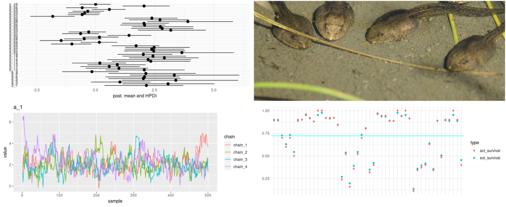
  ggplot(aes(x = key_fct, y = imply, ymin = decrease, ymax = higher)) +
   geom_pointrange() + 
   coord_flip() +  
   xlab("") + ylab("publish. imply and HPDI") +
   theme_minimal() 

Now for an equal to summary. We already computed means, commonplace deviations and the HPDI interval.
Let’s add n_eff, the efficient variety of samples, and rhat, the Gelman-Rubin statistic.

Complete abstract (a.okay.a. “summary”)

is_accepted <- is_accepted %>% as.integer() %>% mean()
step_size <- purrr::map(step_size, imply)

ess <- apply(ess, 2, imply)

summary_with_diag <- abstract %>% add_column(ess = ess, rhat = rhat)
summary_with_diag

# A tibble: 50 x 7
   key    imply    sd  decrease higher   ess  rhat
   <chr> <dbl> <dbl>  <dbl> <dbl> <dbl> <dbl>
 1 a_bar  1.35 0.266  0.792  1.87 405.   1.00
 2 sigma  1.64 0.218  1.23   2.05  83.6  1.00
 3 a_1    2.14 0.887  0.451  3.92  33.5  1.04
 4 a_2    3.16 1.13   1.09   5.48  23.7  1.03
 5 a_3    1.01 0.698 -0.333  2.31  65.2  1.02
 6 a_4    3.02 1.04   1.06   5.05  31.1  1.03
 7 a_5    2.11 0.843  0.625  3.88  49.0  1.05
 8 a_6    2.06 0.904  0.496  3.87  39.8  1.03
 9 a_7    3.20 1.27   1.11   6.12  14.2  1.02
10 a_8    2.21 0.894  0.623  4.18  44.7  1.04
# ... with 40 extra rows

For the various intercepts, efficient pattern sizes are fairly low, indicating we would wish to examine doable causes.

Let’s additionally show posterior survival possibilities, analogously to determine 13.2 within the guide.

Posterior survival possibilities

sim_tanks <- rnorm(8000, a_bar, sigma)
tibble(x = sim_tanks) %>% ggplot(aes(x = x)) + geom_density() + xlab("distribution of per-tank logits")

# our standard sigmoid by one other title (undo the logit)
logistic <- operate(x) 1/(1 + exp(-x))
probs <- map_dbl(sim_tanks, logistic)
tibble(x = probs) %>% ggplot(aes(x = x)) + geom_density() + xlab("chance of survival")

Lastly, we wish to ensure that we see the shrinkage conduct displayed in determine 13.1 within the guide.

Shrinkage

abstract %>% 
  filter(!key %in% c("a_bar", "sigma")) %>%
  choose(key, imply) %>%
  mutate(est_survival = logistic(imply)) %>%
  add_column(act_survival = d$propsurv) %>%
  choose(-imply) %>%
  collect(key = "sort", worth = "worth", -key) %>%
  ggplot(aes(x = key, y = worth, coloration = sort)) +
  geom_point() +
  geom_hline(yintercept = mean(d$propsurv), dimension = 0.5, coloration = "cyan" ) +
  xlab("") +
  ylab("") +
  theme_minimal() +
  theme(axis.textual content.x = element_blank())

We see outcomes related in spirit to McElreath’s: estimates are shrunken to the imply (the cyan-colored line). Additionally, shrinkage appears to be extra lively in smaller tanks, that are the lower-numbered ones on the left of the plot.

Outlook

On this publish, we noticed assemble a various intercepts mannequin with tfprobability, in addition to extract sampling outcomes and related diagnostics. In an upcoming publish, we’ll transfer on to various slopes.
With non-negligible chance, our instance will construct on one in every of Mc Elreath’s once more…
Thanks for studying!