Including uncertainty estimates to Keras fashions with tfprobability

About six months in the past, we confirmed how to create a custom wrapper to acquire uncertainty estimates from a Keras community. Right now we current a much less laborious, as nicely faster-running means utilizing tfprobability, the R wrapper to TensorFlow Chance. Like most posts on this weblog, this one received’t be quick, so let’s rapidly state what you may anticipate in return of studying time.

What to anticipate from this submit

Ranging from what not to anticipate: There received’t be a recipe that tells you the way precisely to set all parameters concerned as a way to report the “proper” uncertainty measures. However then, what are the “proper” uncertainty measures? Except you occur to work with a way that has no (hyper-)parameters to tweak, there’ll all the time be questions on report uncertainty.

What you can anticipate, although, is an introduction to acquiring uncertainty estimates for Keras networks, in addition to an empirical report of how tweaking (hyper-)parameters might have an effect on the outcomes. As within the aforementioned submit, we carry out our assessments on each a simulated and an actual dataset, the Combined Cycle Power Plant Data Set. On the finish, rather than strict guidelines, it is best to have acquired some instinct that can switch to different real-world datasets.

Did you discover our speaking about Keras networks above? Certainly this submit has a further objective: Thus far, we haven’t actually mentioned but how tfprobability goes along with keras. Now we lastly do (briefly: they work collectively seemlessly).

Lastly, the notions of aleatoric and epistemic uncertainty, which can have stayed a bit summary within the prior submit, ought to get way more concrete right here.

Aleatoric vs. epistemic uncertainty

Reminiscent one way or the other of the basic decomposition of generalization error into bias and variance, splitting uncertainty into its epistemic and aleatoric constituents separates an irreducible from a reducible half.

The reducible half pertains to imperfection within the mannequin: In concept, if our mannequin have been good, epistemic uncertainty would vanish. Put otherwise, if the coaching information have been limitless – or in the event that they comprised the entire inhabitants – we might simply add capability to the mannequin till we’ve obtained an ideal match.

In distinction, usually there may be variation in our measurements. There could also be one true course of that determines my resting coronary heart price; nonetheless, precise measurements will fluctuate over time. There’s nothing to be finished about this: That is the aleatoric half that simply stays, to be factored into our expectations.

Now studying this, you is likely to be pondering: “Wouldn’t a mannequin that really have been good seize these pseudo-random fluctuations?”. We’ll go away that phisosophical query be; as an alternative, we’ll attempt to illustrate the usefulness of this distinction by instance, in a sensible means. In a nutshell, viewing a mannequin’s aleatoric uncertainty output ought to warning us to think about applicable deviations when making our predictions, whereas inspecting epistemic uncertainty ought to assist us re-think the appropriateness of the chosen mannequin.

Now let’s dive in and see how we might accomplish our objective with tfprobability. We begin with the simulated dataset.

Uncertainty estimates on simulated information

Dataset

We re-use the dataset from the Google TensorFlow Chance workforce’s blog post on the same subject , with one exception: We prolong the vary of the unbiased variable a bit on the destructive aspect, to raised reveal the completely different strategies’ behaviors.

Right here is the data-generating course of. We additionally get library loading out of the way in which. Just like the previous posts on tfprobability, this one too options not too long ago added performance, so please use the event variations of tensorflow and tfprobability in addition to keras. Name install_tensorflow(model = "nightly") to acquire a present nightly construct of TensorFlow and TensorFlow Chance:

# make certain we use the event variations of tensorflow, tfprobability and keras
devtools::install_github("rstudio/tensorflow")
devtools::install_github("rstudio/tfprobability")
devtools::install_github("rstudio/keras")

# and that we use a nightly construct of TensorFlow and TensorFlow Chance
tensorflow::install_tensorflow(model = "nightly")

library(tensorflow)
library(tfprobability)
library(keras)

library(dplyr)
library(tidyr)
library(ggplot2)

# make certain this code is suitable with TensorFlow 2.0
tf$compat$v1$enable_v2_behavior()

# generate the info
x_min <- -40
x_max <- 60
n <- 150
w0 <- 0.125
b0 <- 5

normalize <- perform(x) (x - x_min) / (x_max - x_min)

# coaching information; predictor 
x <- x_min + (x_max - x_min) * runif(n) %>% as.matrix()

# coaching information; goal
eps <- rnorm(n) * (3 * (0.25 + (normalize(x)) ^ 2))
y <- (w0 * x * (1 + sin(x)) + b0) + eps

# take a look at information (predictor)
x_test <- seq(x_min, x_max, size.out = n) %>% as.matrix()

How does the info look?

ggplot(data.frame(x = x, y = y), aes(x, y)) + geom_point()

Determine 1: Simulated information

The duty right here is single-predictor regression, which in precept we are able to obtain use Keras dense layers.
Let’s see improve this by indicating uncertainty, ranging from the aleatoric sort.

Aleatoric uncertainty

Aleatoric uncertainty, by definition, will not be an announcement concerning the mannequin. So why not have the mannequin be taught the uncertainty inherent within the information?

That is precisely how aleatoric uncertainty is operationalized on this method. As a substitute of a single output per enter – the expected imply of the regression – right here we’ve got two outputs: one for the imply, and one for the usual deviation.

How will we use these? Till shortly, we’d have needed to roll our personal logic. Now with tfprobability, we make the community output not tensors, however distributions – put otherwise, we make the final layer a distribution layer.

Distribution layers are Keras layers, however contributed by tfprobability. The superior factor is that we are able to prepare them with simply tensors as targets, as typical: No have to compute possibilities ourselves.

A number of specialised distribution layers exist, comparable to layer_kl_divergence_add_loss, layer_independent_bernoulli, or layer_mixture_same_family, however essentially the most common is layer_distribution_lambda. layer_distribution_lambda takes as inputs the previous layer and outputs a distribution. So as to have the ability to do that, we have to inform it make use of the previous layer’s activations.

In our case, in some unspecified time in the future we’ll wish to have a dense layer with two models.

... %>% layer_dense(units = 2, activation = "linear") %>%

layer_distribution_lambda(function(x)
    tfd_normal(loc = x[, 1, drop = FALSE],
               scale = 1e-3 + tf$math$softplus(x[, 2, drop = FALSE])
               )
)

model <- keras_model_sequential() %>%
  layer_dense(models = 8, activation = "relu") %>%
  layer_dense(models = 2, activation = "linear") %>%
  layer_distribution_lambda(perform(x)
    tfd_normal(loc = x[, 1, drop = FALSE],
               # ignore on first learn, we'll come again to this
               # scale = 1e-3 + 0.05 * tf$math$softplus(x[, 2, drop = FALSE])
               scale = 1e-3 + tf$math$softplus(x[, 2, drop = FALSE])
               )
  )

For a mannequin that outputs a distribution, the loss is the destructive log probability given the goal information.

negloglik <- perform(y, mannequin) - (mannequin %>% tfd_log_prob(y))

We are able to now compile and match the mannequin.

learning_rate <- 0.01
mannequin %>% compile(optimizer = optimizer_adam(lr = learning_rate), loss = negloglik)

mannequin %>% match(x, y, epochs = 1000)

We now name the mannequin on the take a look at information to acquire the predictions. The predictions now really are distributions, and we’ve got 150 of them, one for every datapoint:

yhat <- mannequin(tf$fixed(x_test))

tfp.distributions.Regular("sequential/distribution_lambda/Regular/",
batch_shape=[150, 1], event_shape=[], dtype=float32)

To acquire the means and commonplace deviations – the latter being that measure of aleatoric uncertainty we’re keen on – we simply name tfd_mean and tfd_stddev on these distributions.
That can give us the expected imply, in addition to the expected variance, per datapoint.

imply <- yhat %>% tfd_mean()
sd <- yhat %>% tfd_stddev()

Let’s visualize this. Listed below are the precise take a look at information factors, the expected means, in addition to confidence bands indicating the imply estimate plus/minus two commonplace deviations.

ggplot(data.frame(
  x = x,
  y = y,
  imply = as.numeric(imply),
  sd = as.numeric(sd)
),
aes(x, y)) +
  geom_point() +
  geom_line(aes(x = x_test, y = imply), shade = "violet", measurement = 1.5) +
  geom_ribbon(aes(
    x = x_test,
    ymin = imply - 2 * sd,
    ymax = imply + 2 * sd
  ),
  alpha = 0.2,
  fill = "gray")

Determine 2: Aleatoric uncertainty on simulated information, utilizing relu activation within the first dense layer.

This appears fairly affordable. What if we had used linear activation within the first layer? Which means, what if the mannequin had appeared like this:

mannequin <- keras_model_sequential() %>%
  layer_dense(models = 8, activation = "linear") %>%
  layer_dense(models = 2, activation = "linear") %>%
  layer_distribution_lambda(perform(x)
    tfd_normal(loc = x[, 1, drop = FALSE],
               scale = 1e-3 + 0.05 * tf$math$softplus(x[, 2, drop = FALSE])
               )
  )

This time, the mannequin doesn’t seize the “type” of the info that nicely, as we’ve disallowed any nonlinearities.

Determine 3: Aleatoric uncertainty on simulated information, utilizing linear activation within the first dense layer.

Utilizing linear activations solely, we additionally have to do extra experimenting with the scale = ... line to get the outcome look “proper”. With relu, then again, outcomes are fairly sturdy to modifications in how scale is computed. Which activation can we select? If our objective is to adequately mannequin variation within the information, we are able to simply select relu – and go away assessing uncertainty within the mannequin to a special approach (the epistemic uncertainty that’s up subsequent).

Total, it looks as if aleatoric uncertainty is the simple half. We would like the community to be taught the variation inherent within the information, which it does. What can we acquire? As a substitute of acquiring simply level estimates, which on this instance may prove fairly dangerous within the two fan-like areas of the info on the left and proper sides, we be taught concerning the unfold as nicely. We’ll thus be appropriately cautious relying on what enter vary we’re making predictions for.

Epistemic uncertainty

Now our focus is on the mannequin. Given a speficic mannequin (e.g., one from the linear household), what sort of information does it say conforms to its expectations?

To reply this query, we make use of a variational-dense layer.
That is once more a Keras layer offered by tfprobability. Internally, it really works by minimizing the proof decrease certain (ELBO), thus striving to search out an approximative posterior that does two issues:

1. match the precise information nicely (put otherwise: obtain excessive log probability), and
2. keep near a prior (as measured by KL divergence).

As customers, we really specify the type of the posterior in addition to that of the prior. Right here is how a previous might look.

prior_trainable <-
  perform(kernel_size,
           bias_size = 0,
           dtype = NULL) {
    n <- kernel_size + bias_size
    keras_model_sequential() %>%
      # we'll touch upon this quickly
      # layer_variable(n, dtype = dtype, trainable = FALSE) %>%
      layer_variable(n, dtype = dtype, trainable = TRUE) %>%
      layer_distribution_lambda(perform(t) {
        tfd_independent(tfd_normal(loc = t, scale = 1),
                        reinterpreted_batch_ndims = 1)
      })
  }

This prior is itself a Keras mannequin, containing a layer that wraps a variable and a layer_distribution_lambda, that sort of distribution-yielding layer we’ve simply encountered above. The variable layer might be mounted (non-trainable) or non-trainable, equivalent to a real prior or a previous learnt from the info in an empirical Bayes-like means. The distribution layer outputs a traditional distribution since we’re in a regression setting.

The posterior too is a Keras mannequin – positively trainable this time. It too outputs a traditional distribution:

posterior_mean_field <-
  perform(kernel_size,
           bias_size = 0,
           dtype = NULL) {
    n <- kernel_size + bias_size
    c <- log(expm1(1))
    keras_model_sequential(list(
      layer_variable(form = 2 * n, dtype = dtype),
      layer_distribution_lambda(
        make_distribution_fn = perform(t) {
          tfd_independent(tfd_normal(
            loc = t[1:n],
            scale = 1e-5 + tf$nn$softplus(c + t[(n + 1):(2 * n)])
            ), reinterpreted_batch_ndims = 1)
        }
      )
    ))
  }

Now that we’ve outlined each, we are able to arrange the mannequin’s layers. The primary one, a variational-dense layer, has a single unit. The following distribution layer then takes that unit’s output and makes use of it for the imply of a traditional distribution – whereas the size of that Regular is mounted at 1:

mannequin <- keras_model_sequential() %>%
  layer_dense_variational(
    models = 1,
    make_posterior_fn = posterior_mean_field,
    make_prior_fn = prior_trainable,
    kl_weight = 1 / n
  ) %>%
  layer_distribution_lambda(perform(x)
    tfd_normal(loc = x, scale = 1))

You might have seen one argument to layer_dense_variational we haven’t mentioned but, kl_weight.
That is used to scale the contribution to the full lack of the KL divergence, and usually ought to equal one over the variety of information factors.

Coaching the mannequin is simple. As customers, we solely specify the destructive log probability a part of the loss; the KL divergence half is taken care of transparently by the framework.

negloglik <- perform(y, mannequin) - (mannequin %>% tfd_log_prob(y))
mannequin %>% compile(optimizer = optimizer_adam(lr = learning_rate), loss = negloglik)
mannequin %>% match(x, y, epochs = 1000)

Due to the stochasticity inherent in a variational-dense layer, every time we name this mannequin, we get hold of completely different outcomes: completely different regular distributions, on this case.
To acquire the uncertainty estimates we’re in search of, we due to this fact name the mannequin a bunch of occasions – 100, say:

yhats <- purrr::map(1:100, perform(x) mannequin(tf$fixed(x_test)))

We are able to now plot these 100 predictions – strains, on this case, as there aren’t any nonlinearities:

means <-
  purrr::map(yhats, purrr::compose(as.matrix, tfd_mean)) %>% abind::abind()

strains <- data.frame(cbind(x_test, means)) %>%
  collect(key = run, worth = worth,-X1)

imply <- apply(means, 1, imply)

ggplot(data.frame(x = x, y = y, imply = as.numeric(imply)), aes(x, y)) +
  geom_point() +
  geom_line(aes(x = x_test, y = imply), shade = "violet", measurement = 1.5) +
  geom_line(
    information = strains,
    aes(x = X1, y = worth, shade = run),
    alpha = 0.3,
    measurement = 0.5
  ) +
  theme(legend.place = "none")

Determine 4: Epistemic uncertainty on simulated information, utilizing linear activation within the variational-dense layer.

What we see listed below are basically completely different fashions, in step with the assumptions constructed into the structure. What we’re not accounting for is the unfold within the information. Can we do each? We are able to; however first let’s touch upon a couple of selections that have been made and see how they have an effect on the outcomes.

To forestall this submit from rising to infinite measurement, we’ve avoided performing a scientific experiment; please take what follows not as generalizable statements, however as tips that could issues you’ll want to be mindful in your personal ventures. Particularly, every (hyper-)parameter will not be an island; they might work together in unexpected methods.

After these phrases of warning, listed below are some issues we seen.

1. One query you may ask: Earlier than, within the aleatoric uncertainty setup, we added a further dense layer to the mannequin, with relu activation. What if we did this right here?
   Firstly, we’re not including any extra, non-variational layers as a way to hold the setup “totally Bayesian” – we wish priors at each stage. As to utilizing relu in layer_dense_variational, we did attempt that, and the outcomes look fairly related:

Determine 5: Epistemic uncertainty on simulated information, utilizing relu activation within the variational-dense layer.

Nevertheless, issues look fairly completely different if we drastically cut back coaching time… which brings us to the subsequent commentary.

2. Not like within the aleatoric setup, the variety of coaching epochs matter loads. If we prepare, quote unquote, too lengthy, the posterior estimates will get nearer and nearer to the posterior imply: we lose uncertainty. What occurs if we prepare “too quick” is much more notable. Listed below are the outcomes for the linear-activation in addition to the relu-activation instances:

Determine 6: Epistemic uncertainty on simulated information if we prepare for 100 epochs solely. Left: linear activation. Proper: relu activation.

Apparently, each mannequin households look very completely different now, and whereas the linear-activation household appears extra affordable at first, it nonetheless considers an general destructive slope in step with the info.

So what number of epochs are “lengthy sufficient”? From commentary, we’d say {that a} working heuristic ought to most likely be based mostly on the speed of loss discount. However definitely, it’ll make sense to attempt completely different numbers of epochs and test the impact on mannequin conduct. As an apart, monitoring estimates over coaching time might even yield necessary insights into the assumptions constructed right into a mannequin (e.g., the impact of various activation capabilities).

3. As necessary because the variety of epochs educated, and related in impact, is the studying price. If we substitute the educational price on this setup by 0.001, outcomes will look just like what we noticed above for the epochs = 100 case. Once more, we’ll wish to attempt completely different studying charges and ensure we prepare the mannequin “to completion” in some affordable sense.

4. To conclude this part, let’s rapidly take a look at what occurs if we fluctuate two different parameters. What if the prior have been non-trainable (see the commented line above)? And what if we scaled the significance of the KL divergence (kl_weight in layer_dense_variational’s argument listing) otherwise, changing kl_weight = 1/n by kl_weight = 1 (or equivalently, eradicating it)? Listed below are the respective outcomes for an otherwise-default setup. They don’t lend themselves to generalization – on completely different (e.g., greater!) datasets the outcomes will most definitely look completely different – however positively fascinating to watch.

Determine 7: Epistemic uncertainty on simulated information. Left: kl_weight = 1. Proper: prior non-trainable.

Now let’s come again to the query: We’ve modeled unfold within the information, we’ve peeked into the center of the mannequin, – can we do each on the identical time?

We are able to, if we mix each approaches. We add a further unit to the variational-dense layer and use this to be taught the variance: as soon as for every “sub-model” contained within the mannequin.

Combining each aleatoric and epistemic uncertainty

Reusing the prior and posterior from above, that is how the ultimate mannequin appears:

mannequin <- keras_model_sequential() %>%
  layer_dense_variational(
    models = 2,
    make_posterior_fn = posterior_mean_field,
    make_prior_fn = prior_trainable,
    kl_weight = 1 / n
  ) %>%
  layer_distribution_lambda(perform(x)
    tfd_normal(loc = x[, 1, drop = FALSE],
               scale = 1e-3 + tf$math$softplus(0.01 * x[, 2, drop = FALSE])
               )
    )

We prepare this mannequin identical to the epistemic-uncertainty just one. We then get hold of a measure of uncertainty per predicted line. Or within the phrases we used above, we now have an ensemble of fashions every with its personal indication of unfold within the information. Here’s a means we might show this – every coloured line is the imply of a distribution, surrounded by a confidence band indicating +/- two commonplace deviations.

yhats <- purrr::map(1:100, perform(x) mannequin(tf$fixed(x_test)))
means <-
  purrr::map(yhats, purrr::compose(as.matrix, tfd_mean)) %>% abind::abind()
sds <-
  purrr::map(yhats, purrr::compose(as.matrix, tfd_stddev)) %>% abind::abind()

means_gathered <- data.frame(cbind(x_test, means)) %>%
  collect(key = run, worth = mean_val,-X1)
sds_gathered <- data.frame(cbind(x_test, sds)) %>%
  collect(key = run, worth = sd_val,-X1)

strains <-
  means_gathered %>% inner_join(sds_gathered, by = c("X1", "run"))
imply <- apply(means, 1, imply)

ggplot(data.frame(x = x, y = y, imply = as.numeric(imply)), aes(x, y)) +
  geom_point() +
  theme(legend.place = "none") +
  geom_line(aes(x = x_test, y = imply), shade = "violet", measurement = 1.5) +
  geom_line(
    information = strains,
    aes(x = X1, y = mean_val, shade = run),
    alpha = 0.6,
    measurement = 0.5
  ) +
  geom_ribbon(
    information = strains,
    aes(
      x = X1,
      ymin = mean_val - 2 * sd_val,
      ymax = mean_val + 2 * sd_val,
      group = run
    ),
    alpha = 0.05,
    fill = "gray",
    inherit.aes = FALSE
  )

Determine 8: Displaying each epistemic and aleatoric uncertainty on the simulated dataset.

Good! This appears like one thing we might report.

As you may think, this mannequin, too, is delicate to how lengthy (suppose: variety of epochs) or how briskly (suppose: studying price) we prepare it. And in comparison with the epistemic-uncertainty solely mannequin, there may be a further option to be made right here: the scaling of the earlier layer’s activation – the 0.01 within the scale argument to tfd_normal:

scale = 1e-3 + tf$math$softplus(0.01 * x[, 2, drop = FALSE])

Protecting all the pieces else fixed, right here we fluctuate that parameter between 0.01 and 0.05:

Determine 9: Epistemic plus aleatoric uncertainty on the simulated dataset: Various the size argument.

Evidently, that is one other parameter we needs to be ready to experiment with.

Now that we’ve launched all three sorts of presenting uncertainty – aleatoric solely, epistemic solely, or each – let’s see them on the aforementioned Combined Cycle Power Plant Data Set. Please see our previous post on uncertainty for a fast characterization, in addition to visualization, of the dataset.

Mixed Cycle Energy Plant Knowledge Set

To maintain this submit at a digestible size, we’ll chorus from making an attempt as many alternate options as with the simulated information and primarily stick with what labored nicely there. This also needs to give us an thought of how nicely these “defaults” generalize. We individually examine two situations: The only-predictor setup (utilizing every of the 4 accessible predictors alone), and the entire one (utilizing all 4 predictors directly).

The dataset is loaded simply as within the earlier submit.

First we take a look at the single-predictor case, ranging from aleatoric uncertainty.

Single predictor: Aleatoric uncertainty

Right here is the “default” aleatoric mannequin once more. We additionally duplicate the plotting code right here for the reader’s comfort.

n <- nrow(X_train) # 7654
n_epochs <- 10 # we'd like fewer epochs as a result of the dataset is a lot greater

batch_size <- 100

learning_rate <- 0.01

# variable to suit - change to 2,3,4 to get the opposite predictors
i <- 1

mannequin <- keras_model_sequential() %>%
  layer_dense(models = 16, activation = "relu") %>%
  layer_dense(models = 2, activation = "linear") %>%
  layer_distribution_lambda(perform(x)
    tfd_normal(loc = x[, 1, drop = FALSE],
               scale = tf$math$softplus(x[, 2, drop = FALSE])
               )
    )

negloglik <- perform(y, mannequin) - (mannequin %>% tfd_log_prob(y))

mannequin %>% compile(optimizer = optimizer_adam(lr = learning_rate), loss = negloglik)

hist <-
  mannequin %>% match(
    X_train[, i, drop = FALSE],
    y_train,
    validation_data = list(X_val[, i, drop = FALSE], y_val),
    epochs = n_epochs,
    batch_size = batch_size
  )

yhat <- mannequin(tf$fixed(X_val[, i, drop = FALSE]))

imply <- yhat %>% tfd_mean()
sd <- yhat %>% tfd_stddev()

ggplot(data.frame(
  x = X_val[, i],
  y = y_val,
  imply = as.numeric(imply),
  sd = as.numeric(sd)
),
aes(x, y)) +
  geom_point() +
  geom_line(aes(x = x, y = imply), shade = "violet", measurement = 1.5) +
  geom_ribbon(aes(
    x = x,
    ymin = imply - 2 * sd,
    ymax = imply + 2 * sd
  ),
  alpha = 0.4,
  fill = "gray")

How nicely does this work?

Determine 10: Aleatoric uncertainty on the Mixed Cycle Energy Plant Knowledge Set; single predictors.

This appears fairly good we’d say! How about epistemic uncertainty?

Single predictor: Epistemic uncertainty

Right here’s the code:

posterior_mean_field <-
  perform(kernel_size,
           bias_size = 0,
           dtype = NULL) {
    n <- kernel_size + bias_size
    c <- log(expm1(1))
    keras_model_sequential(list(
      layer_variable(form = 2 * n, dtype = dtype),
      layer_distribution_lambda(
        make_distribution_fn = perform(t) {
          tfd_independent(tfd_normal(
            loc = t[1:n],
            scale = 1e-5 + tf$nn$softplus(c + t[(n + 1):(2 * n)])
          ), reinterpreted_batch_ndims = 1)
        }
      )
    ))
  }

prior_trainable <-
  perform(kernel_size,
           bias_size = 0,
           dtype = NULL) {
    n <- kernel_size + bias_size
    keras_model_sequential() %>%
      layer_variable(n, dtype = dtype, trainable = TRUE) %>%
      layer_distribution_lambda(perform(t) {
        tfd_independent(tfd_normal(loc = t, scale = 1),
                        reinterpreted_batch_ndims = 1)
      })
  }

mannequin <- keras_model_sequential() %>%
  layer_dense_variational(
    models = 1,
    make_posterior_fn = posterior_mean_field,
    make_prior_fn = prior_trainable,
    kl_weight = 1 / n,
    activation = "linear",
  ) %>%
  layer_distribution_lambda(perform(x)
    tfd_normal(loc = x, scale = 1))

negloglik <- perform(y, mannequin) - (mannequin %>% tfd_log_prob(y))
mannequin %>% compile(optimizer = optimizer_adam(lr = learning_rate), loss = negloglik)
hist <-
  mannequin %>% match(
    X_train[, i, drop = FALSE],
    y_train,
    validation_data = list(X_val[, i, drop = FALSE], y_val),
    epochs = n_epochs,
    batch_size = batch_size
  )

yhats <- purrr::map(1:100, perform(x)
  yhat <- mannequin(tf$fixed(X_val[, i, drop = FALSE])))
  
means <-
  purrr::map(yhats, purrr::compose(as.matrix, tfd_mean)) %>% abind::abind()

strains <- data.frame(cbind(X_val[, i], means)) %>%
  collect(key = run, worth = worth,-X1)

imply <- apply(means, 1, imply)
ggplot(data.frame(x = X_val[, i], y = y_val, imply = as.numeric(imply)), aes(x, y)) +
  geom_point() +
  geom_line(aes(x = X_val[, i], y = imply), shade = "violet", measurement = 1.5) +
  geom_line(
    information = strains,
    aes(x = X1, y = worth, shade = run),
    alpha = 0.3,
    measurement = 0.5
  ) +
  theme(legend.place = "none")

And that is the outcome.

Determine 11: Epistemic uncertainty on the Mixed Cycle Energy Plant Knowledge Set; single predictors.

As with the simulated information, the linear fashions appears to “do the best factor”. And right here too, we expect we’ll wish to increase this with the unfold within the information: Thus, on to means three.

Single predictor: Combining each sorts

Right here we go. Once more, posterior_mean_field and prior_trainable look identical to within the epistemic-only case.

mannequin <- keras_model_sequential() %>%
  layer_dense_variational(
    models = 2,
    make_posterior_fn = posterior_mean_field,
    make_prior_fn = prior_trainable,
    kl_weight = 1 / n,
    activation = "linear"
  ) %>%
  layer_distribution_lambda(perform(x)
    tfd_normal(loc = x[, 1, drop = FALSE],
               scale = 1e-3 + tf$math$softplus(0.01 * x[, 2, drop = FALSE])))


negloglik <- perform(y, mannequin)
  - (mannequin %>% tfd_log_prob(y))
mannequin %>% compile(optimizer = optimizer_adam(lr = learning_rate), loss = negloglik)
hist <-
  mannequin %>% match(
    X_train[, i, drop = FALSE],
    y_train,
    validation_data = list(X_val[, i, drop = FALSE], y_val),
    epochs = n_epochs,
    batch_size = batch_size
  )

yhats <- purrr::map(1:100, perform(x)
  mannequin(tf$fixed(X_val[, i, drop = FALSE])))
means <-
  purrr::map(yhats, purrr::compose(as.matrix, tfd_mean)) %>% abind::abind()
sds <-
  purrr::map(yhats, purrr::compose(as.matrix, tfd_stddev)) %>% abind::abind()

means_gathered <- data.frame(cbind(X_val[, i], means)) %>%
  collect(key = run, worth = mean_val,-X1)
sds_gathered <- data.frame(cbind(X_val[, i], sds)) %>%
  collect(key = run, worth = sd_val,-X1)

strains <-
  means_gathered %>% inner_join(sds_gathered, by = c("X1", "run"))

imply <- apply(means, 1, imply)

#strains <- strains %>% filter(run=="X3" | run =="X4")

ggplot(data.frame(x = X_val[, i], y = y_val, imply = as.numeric(imply)), aes(x, y)) +
  geom_point() +
  theme(legend.place = "none") +
  geom_line(aes(x = X_val[, i], y = imply), shade = "violet", measurement = 1.5) +
  geom_line(
    information = strains,
    aes(x = X1, y = mean_val, shade = run),
    alpha = 0.2,
    measurement = 0.5
  ) +
geom_ribbon(
  information = strains,
  aes(
    x = X1,
    ymin = mean_val - 2 * sd_val,
    ymax = mean_val + 2 * sd_val,
    group = run
  ),
  alpha = 0.01,
  fill = "gray",
  inherit.aes = FALSE
)

And the output?

Determine 12: Mixed uncertainty on the Mixed Cycle Energy Plant Knowledge Set; single predictors.

This appears helpful! Let’s wrap up with our remaining take a look at case: Utilizing all 4 predictors collectively.

All predictors

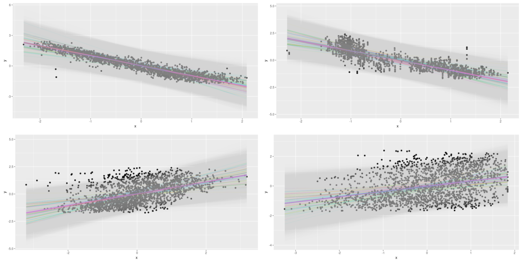
The coaching code used on this situation appears identical to earlier than, other than our feeding all predictors to the mannequin. For plotting, we resort to displaying the primary principal element on the x-axis – this makes the plots look noisier than earlier than. We additionally show fewer strains for the epistemic and epistemic-plus-aleatoric instances (20 as an alternative of 100). Listed below are the outcomes:

Determine 13: Uncertainty (aleatoric, epistemic, each) on the Mixed Cycle Energy Plant Knowledge Set; all predictors.

Conclusion

The place does this go away us? In comparison with the learnable-dropout method described within the prior submit, the way in which introduced here’s a lot simpler, quicker, and extra intuitively comprehensible.
The strategies per se are that straightforward to make use of that on this first introductory submit, we might afford to discover alternate options already: one thing we had no time to do in that earlier exposition.

In truth, we hope this submit leaves you ready to do your personal experiments, by yourself information.
Clearly, you’ll have to make selections, however isn’t that the way in which it’s in information science? There’s no means round making selections; we simply needs to be ready to justify them …
Thanks for studying!