Dynamic linear fashions with tfprobability
Welcome to the world of state area fashions. On this world, there’s a latent course of, hidden from our eyes; and there are observations we make concerning the issues it produces. The method evolves attributable to some hidden logic (transition mannequin); and the way in which it produces the observations follows some hidden logic (remark mannequin). There’s noise in course of evolution, and there may be noise in remark. If the transition and remark fashions each are linear, and the method in addition to remark noise are Gaussian, we’ve got a linear-Gaussian state area mannequin (SSM). The duty is to deduce the latent state from the observations. Probably the most well-known approach is the Kálmán filter.
In sensible purposes, two traits of linear-Gaussian SSMs are particularly engaging.
For one, they allow us to estimate dynamically altering parameters. In regression, the parameters will be considered as a hidden state; we might thus have a slope and an intercept that fluctuate over time. When parameters can range, we communicate of dynamic linear fashions (DLMs). That is the time period we’ll use all through this submit when referring to this class of fashions.
Second, linear-Gaussian SSMs are helpful in time-series forecasting as a result of Gaussian processes will be added. A time sequence can thus be framed as, e.g. the sum of a linear pattern and a course of that varies seasonally.
Utilizing tfprobability, the R wrapper to TensorFlow Likelihood, we illustrate each points right here. Our first instance can be on dynamic linear regression. In an in depth walkthrough, we present on tips on how to match such a mannequin, tips on how to receive filtered, in addition to smoothed, estimates of the coefficients, and tips on how to receive forecasts.
Our second instance then illustrates course of additivity. This instance will construct on the primary, and may additionally function a fast recap of the general process.
Let’s leap in.
Dynamic linear regression instance: Capital Asset Pricing Mannequin (CAPM)
Our code builds on the not too long ago launched variations of TensorFlow and TensorFlow Likelihood: 1.14 and 0.7, respectively.
Word how there’s one factor we used to do these days that we’re not doing right here: We’re not enabling keen execution. We are saying why in a minute.
Our instance is taken from Petris et al.(2009)(Petris, Petrone, and Campagnoli 2009), chapter 3.2.7.
In addition to introducing the dlm bundle, this ebook gives a pleasant introduction to the concepts behind DLMs typically.
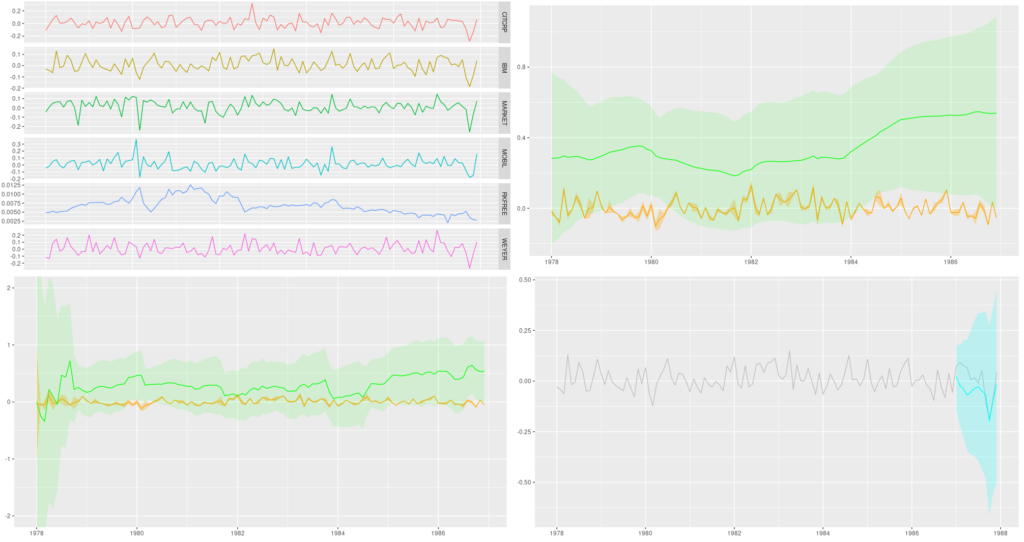
As an instance dynamic linear regression, the authors function a dataset, initially from Berndt(1991)(Berndt 1991) that has month-to-month returns, collected from January 1978 to December 1987, for 4 totally different shares, the 30-day Treasury Invoice – standing in for a risk-free asset –, and the value-weighted common returns for all shares listed on the New York and American Inventory Exchanges, representing the general market returns.
Let’s have a look.
# As the info doesn't appear to be accessible on the tackle given in Petris et al. any extra,
# we put it on the weblog for obtain
# obtain from:
# https://github.com/rstudio/tensorflow-blog/blob/grasp/docs/posts/2019-06-25-dynamic_linear_models_tfprobability/knowledge/capm.txt"
df <- read_table(
  "capm.txt",
  col_types = list(X1 = col_date(format = "%Y.%m"))) %>%
  rename(month = X1)
df %>% glimpse()
Observations: 120
Variables: 7
$ month <date> 1978-01-01, 1978-02-01, 1978-03-01, 1978-04-01, 1978-05-01, 19…
$ MOBIL <dbl> -0.046, -0.017, 0.049, 0.077, -0.011, -0.043, 0.028, 0.056, 0.0…
$ IBM <dbl> -0.029, -0.043, -0.063, 0.130, -0.018, -0.004, 0.092, 0.049, -0…
$ WEYER <dbl> -0.116, -0.135, 0.084, 0.144, -0.031, 0.005, 0.164, 0.039, -0.0…
$ CITCRP <dbl> -0.115, -0.019, 0.059, 0.127, 0.005, 0.007, 0.032, 0.088, 0.011…
$ MARKET <dbl> -0.045, 0.010, 0.050, 0.063, 0.067, 0.007, 0.071, 0.079, 0.002,…
$ RKFREE <dbl> 0.00487, 0.00494, 0.00526, 0.00491, 0.00513, 0.00527, 0.00528, …df %>% collect(key = "image", worth = "return", -month) %>%
ggplot(aes(x = month, y = return, colour = image)) +
geom_line() +
facet_grid(rows = vars(image), scales = "free")
Determine 1: Month-to-month returns for chosen shares; knowledge from Berndt (1991).
The Capital Asset Pricing Model then assumes a linear relationship between the surplus returns of an asset beneath research and the surplus returns of the market. For each, extra returns are obtained by subtracting the returns of the chosen risk-free asset; then, the scaling coefficient between them reveals the asset to both be an “aggressive” funding (slope > 1: modifications out there are amplified), or a conservative one (slope < 1: modifications are damped).
Assuming this relationship doesn’t change over time, we are able to simply use lm as an instance this. Following Petris et al. in zooming in on IBM because the asset beneath research, we’ve got
Name:
lm(method = ibm ~ x)

Residuals:
     Min       1Q   Median       3Q      Max
-0.11850 -0.03327 -0.00263  0.03332  0.15042

Coefficients:
              Estimate Std. Error t worth Pr(>|t|)
(Intercept) -0.0004896  0.0046400  -0.106    0.916
x            0.4568208  0.0675477   6.763 5.49e-10 ***
---
Signif. codes:  0 ‘***’ 0.001 ‘**’ 0.01 ‘*’ 0.05 ‘.’ 0.1 ‘ ’ 1

Residual commonplace error: 0.05055 on 118 levels of freedom
A number of R-squared:  0.2793,    Adjusted R-squared:  0.2732
F-statistic: 45.74 on 1 and 118 DF,  p-value: 5.489e-10
So IBM is discovered to be a conservative funding, the slope being ~ 0.5. However is that this relationship secure over time?
Let’s flip to tfprobability to research.
We wish to use this instance to display two important purposes of DLMs: acquiring smoothing and/or filtering estimates of the coefficients, in addition to forecasting future values. So in contrast to Petris et al., we divide the dataset right into a coaching and a testing half:.
We now assemble the mannequin. sts_dynamic_linear_regression() does what we would like:
We go it the column of extra market returns, plus a column of ones, following Petris et al.. Alternatively, we may middle the only predictor – this is able to work simply as properly.
How are we going to coach this mannequin? Methodology-wise, we’ve got a alternative between variational inference (VI) and Hamiltonian Monte Carlo (HMC). We’ll see each. The second query is: Are we going to make use of graph mode or keen mode? As of as we speak, for each VI and HMC, it’s most secure – and quickest – to run in graph mode, so that is the one approach we present. In a number of weeks, or months, we must always be capable to prune plenty of sess$run()s from the code!
Usually in posts, when presenting code we optimize for straightforward experimentation (that means: line-by-line executability), not modularity. This time although, with an necessary variety of analysis statements concerned, it’s best to pack not simply the becoming, however the smoothing and forecasting as properly right into a operate (which you might nonetheless step via when you wished). For VI, we’ll have a match _with_vi operate that does all of it. So after we now begin explaining what it does, don’t sort within the code simply but – it’ll all reappear properly packed into that operate, so that you can copy and execute as a complete.
Becoming a time sequence with variational inference
Becoming with VI just about appears like coaching historically used to look in graph-mode TensorFlow. You outline a loss – right here it’s achieved utilizing sts_build_factored_variational_loss() –, an optimizer, and an operation for the optimizer to scale back that loss:
optimizer <- tf$compat$v1$practice$AdamOptimizer(0.1)

# solely practice on the coaching set!
loss_and_dists <- ts_train %>% sts_build_factored_variational_loss(mannequin = mannequin)
variational_loss <- loss_and_dists[[1]]

train_op <- optimizer$reduce(variational_loss)
Word how the loss is outlined on the coaching set solely, not the whole sequence.
Now to really practice the mannequin, we create a session and run that operation:
 with (tf$Session() %as% sess,  {

      sess$run(tf$compat$v1$global_variables_initializer())

      for (step in 1:n_iterations) {
        res <- sess$run(train_op)
        loss <- sess$run(variational_loss)
        if (step %% 10 == 0)
          cat("Loss: ", as.numeric(loss), "n")
      }
 })
Given we’ve got that session, let’s make use of it and compute all of the estimates we want.
Once more, – the next snippets will find yourself within the fit_with_vi operate, so don’t run them in isolation simply but.
Acquiring forecasts
The very first thing we would like for the mannequin to offer us are forecasts. So as to create them, it wants samples from the posterior. Fortunately we have already got the posterior distributions, returned from sts_build_factored_variational_loss, so let’s pattern from them and go them to sts_forecast:
sts_forecast() returns distributions, so we name tfd_mean() to get the posterior predictions and tfd_stddev() for the corresponding commonplace deviations:
fc_means <- forecast_dists %>% tfd_mean()
fc_sds <- forecast_dists %>% tfd_stddev()By the way in which – as we’ve got the complete posterior distributions, we’re certainly not restricted to abstract statistics! We may simply use tfd_sample() to acquire particular person forecasts.
Smoothing and filtering (Kálmán filter)
Now, the second (and final, for this instance) factor we’ll need are the smoothed and filtered regression coefficients. The well-known Kálmán Filter is a Bayesian-in-spirit technique the place at every time step, predictions are corrected by how a lot they differ from an incoming remark. Filtering estimates are based mostly on observations we’ve seen up to now; smoothing estimates are computed “in hindsight,” making use of the whole time sequence.
We first create a state area mannequin from our time sequence definition:
# solely do that on the coaching set
# returns an occasion of tfd_linear_gaussian_state_space_model()
ssm <- mannequin$make_state_space_model(length(ts_train), param_vals = posterior_samples)tfd_linear_gaussian_state_space_model(), technically a distribution, gives the Kálmán filter functionalities of smoothing and filtering.
To acquire the smoothed estimates:
c(smoothed_means, smoothed_covs) %<-% ssm$posterior_marginals(ts_train)And the filtered ones:
c(., filtered_means, filtered_covs, ., ., ., .) %<-% ssm$forward_filter(ts_train)Lastly, we have to consider all these.
Placing all of it collectively (the VI version)
So right here’s the whole operate, fit_with_vi, prepared for us to name.
fit_with_vi <-
operate(ts,
ts_train,
mannequin,
n_iterations,
n_param_samples,
n_forecast_steps,
n_forecast_samples) {
optimizer <- tf$compat$v1$practice$AdamOptimizer(0.1)
loss_and_dists <-
ts_train %>% sts_build_factored_variational_loss(mannequin = mannequin)
variational_loss <- loss_and_dists[[1]]
train_op <- optimizer$reduce(variational_loss)
with (tf$Session() %as% sess, {
sess$run(tf$compat$v1$global_variables_initializer())
for (step in 1:n_iterations) {
sess$run(train_op)
loss <- sess$run(variational_loss)
if (step %% 1 == 0)
cat("Loss: ", as.numeric(loss), "n")
}
variational_distributions <- loss_and_dists[[2]]
posterior_samples <-
  Map(
    operate(d) d %>% tfd_sample(n_param_samples),
    variational_distributions %>% reticulate::py_to_r() %>% unname()
  )
forecast_dists <- ts_train %>% sts_forecast(mannequin, posterior_samples, n_forecast_steps)
fc_means <- forecast_dists %>% tfd_mean()
fc_sds <- forecast_dists %>% tfd_stddev()
ssm <- mannequin$make_state_space_model(length(ts_train), param_vals = posterior_samples)
c(smoothed_means, smoothed_covs) %<-% ssm$posterior_marginals(ts_train)
c(., filtered_means, filtered_covs, ., ., ., .) %<-% ssm$forward_filter(ts_train)
c(posterior_samples, fc_means, fc_sds, smoothed_means, smoothed_covs, filtered_means, filtered_covs) %<-%
  sess$run(list(posterior_samples, fc_means, fc_sds, smoothed_means, smoothed_covs, filtered_means, filtered_covs))
})
list(
variational_distributions,
posterior_samples,
fc_means[, 1],
fc_sds[, 1],
smoothed_means,
smoothed_covs,
filtered_means,
filtered_covs
)
}And that is how we name it.
# variety of VI steps
n_iterations <- 300
# pattern dimension for posterior samples
n_param_samples <- 50
# pattern dimension to attract from the forecast distribution
n_forecast_samples <- 50

# here is the mannequin once more
mannequin <- ts %>%
  sts_dynamic_linear_regression(design_matrix = cbind(rep(1, length(x)), x) %>% tf$solid(tf$float32))

# name fit_vi outlined above
c(
  param_distributions,
  param_samples,
  fc_means,
  fc_sds,
  smoothed_means,
  smoothed_covs,
  filtered_means,
  filtered_covs
) %<-% fit_vi(
  ts,
  ts_train,
  mannequin,
  n_iterations,
  n_param_samples,
  n_forecast_steps,
  n_forecast_samples
)
Curious concerning the outcomes? We’ll see them in a second, however earlier than let’s simply shortly look on the various coaching technique: HMC.
Placing all of it collectively (the HMC version)
tfprobability gives sts_fit_with_hmc to suit a DLM utilizing Hamiltonian Monte Carlo. Current posts (e.g., Hierarchical partial pooling, continued: Varying slopes models with TensorFlow Probability) confirmed tips on how to arrange HMC to suit hierarchical fashions; right here a single operate does all of it.
Right here is fit_with_hmc, wrapping sts_fit_with_hmc in addition to the (unchanged) strategies for acquiring forecasts and smoothed/filtered parameters:
num_results <- 200
num_warmup_steps <- 100

fit_hmc <- operate(ts,
                    ts_train,
                    mannequin,
                    num_results,
                    num_warmup_steps,
                    n_forecast,
                    n_forecast_samples) {

  states_and_results <-
    ts_train %>% sts_fit_with_hmc(
      mannequin,
      num_results = num_results,
      num_warmup_steps = num_warmup_steps,
      num_variational_steps = num_results + num_warmup_steps
    )

  posterior_samples <- states_and_results[[1]]
  forecast_dists <-
    ts_train %>% sts_forecast(mannequin, posterior_samples, n_forecast_steps)
  fc_means <- forecast_dists %>% tfd_mean()
  fc_sds <- forecast_dists %>% tfd_stddev()

  ssm <-
    mannequin$make_state_space_model(length(ts_train), param_vals = posterior_samples)
  c(smoothed_means, smoothed_covs) %<-% ssm$posterior_marginals(ts_train)
  c(., filtered_means, filtered_covs, ., ., ., .) %<-% ssm$forward_filter(ts_train)

  with (tf$Session() %as% sess,  {
    sess$run(tf$compat$v1$global_variables_initializer())
    c(
      posterior_samples,
      fc_means,
      fc_sds,
      smoothed_means,
      smoothed_covs,
      filtered_means,
      filtered_covs
    ) %<-%
      sess$run(
        list(
          posterior_samples,
          fc_means,
          fc_sds,
          smoothed_means,
          smoothed_covs,
          filtered_means,
          filtered_covs
        )
      )
  })

  list(
    posterior_samples,
    fc_means[, 1],
    fc_sds[, 1],
    smoothed_means,
    smoothed_covs,
    filtered_means,
    filtered_covs
  )
}

c(
  param_samples,
  fc_means,
  fc_sds,
  smoothed_means,
  smoothed_covs,
  filtered_means,
  filtered_covs
) %<-% fit_hmc(ts,
               ts_train,
               mannequin,
               num_results,
               num_warmup_steps,
               n_forecast,
               n_forecast_samples)
Now lastly, let’s check out the forecasts and filtering resp. smoothing estimates.
Forecasts
Placing all we’d like into one dataframe, we’ve got
smoothed_means_intercept <- smoothed_means[, , 1] %>% colMeans()
smoothed_means_slope <- smoothed_means[, , 2] %>% colMeans()

smoothed_sds_intercept <- smoothed_covs[, , 1, 1] %>% colMeans() %>% sqrt()
smoothed_sds_slope <- smoothed_covs[, , 2, 2] %>% colMeans() %>% sqrt()

filtered_means_intercept <- filtered_means[, , 1] %>% colMeans()
filtered_means_slope <- filtered_means[, , 2] %>% colMeans()

filtered_sds_intercept <- filtered_covs[, , 1, 1] %>% colMeans() %>% sqrt()
filtered_sds_slope <- filtered_covs[, , 2, 2] %>% colMeans() %>% sqrt()

forecast_df <- df %>%
  choose(month, IBM) %>%
  add_column(pred_mean = c(rep(NA, length(ts_train)), fc_means)) %>%
  add_column(pred_sd = c(rep(NA, length(ts_train)), fc_sds)) %>%
  add_column(smoothed_means_intercept = c(smoothed_means_intercept, rep(NA, n_forecast_steps))) %>%
  add_column(smoothed_means_slope = c(smoothed_means_slope, rep(NA, n_forecast_steps))) %>%
  add_column(smoothed_sds_intercept = c(smoothed_sds_intercept, rep(NA, n_forecast_steps))) %>%
  add_column(smoothed_sds_slope = c(smoothed_sds_slope, rep(NA, n_forecast_steps))) %>%
  add_column(filtered_means_intercept = c(filtered_means_intercept, rep(NA, n_forecast_steps))) %>%
  add_column(filtered_means_slope = c(filtered_means_slope, rep(NA, n_forecast_steps))) %>%
  add_column(filtered_sds_intercept = c(filtered_sds_intercept, rep(NA, n_forecast_steps))) %>%
  add_column(filtered_sds_slope = c(filtered_sds_slope, rep(NA, n_forecast_steps)))
So right here first are the forecasts. We’re utilizing the estimates returned from VI, however we may simply as properly have used these from HMC – they’re almost indistinguishable. The identical goes for the filtering and smoothing estimates displayed beneath.
ggplot(forecast_df, aes(x = month, y = IBM)) +
  geom_line(colour = "gray") +
  geom_line(aes(y = pred_mean), colour = "cyan") +
  geom_ribbon(
    aes(ymin = pred_mean - 2 * pred_sd, ymax = pred_mean + 2 * pred_sd),
    alpha = 0.2,
    fill = "cyan"
  ) +
  theme(axis.title = element_blank())
Determine 2: 12-point-ahead forecasts for IBM; posterior means +/- 2 commonplace deviations.
Smoothing estimates
Listed here are the smoothing estimates. The intercept (proven in orange) stays fairly secure over time, however we do see a pattern within the slope (displayed in inexperienced).
ggplot(forecast_df, aes(x = month, y = smoothed_means_intercept)) +
  geom_line(colour = "orange") +
  geom_line(aes(y = smoothed_means_slope),
            colour = "inexperienced") +
  geom_ribbon(
    aes(
      ymin = smoothed_means_intercept - 2 * smoothed_sds_intercept,
      ymax = smoothed_means_intercept + 2 * smoothed_sds_intercept
    ),
    alpha = 0.3,
    fill = "orange"
  ) +
  geom_ribbon(
    aes(
      ymin = smoothed_means_slope - 2 * smoothed_sds_slope,
      ymax = smoothed_means_slope + 2 * smoothed_sds_slope
    ),
    alpha = 0.1,
    fill = "inexperienced"
  ) +
  coord_cartesian(xlim = c(forecast_df$month[1], forecast_df$month[length(ts) - n_forecast_steps]))  +
  theme(axis.title = element_blank())
Determine 3: Smoothing estimates from the Kálmán filter. Inexperienced: coefficient for dependence on extra market returns (slope), orange: vector of ones (intercept).
Filtering estimates
For comparability, listed here are the filtering estimates. Word that the y-axis extends additional up and down, so we are able to seize uncertainty higher:
ggplot(forecast_df, aes(x = month, y = filtered_means_intercept)) +
  geom_line(colour = "orange") +
  geom_line(aes(y = filtered_means_slope),
            colour = "inexperienced") +
  geom_ribbon(
    aes(
      ymin = filtered_means_intercept - 2 * filtered_sds_intercept,
      ymax = filtered_means_intercept + 2 * filtered_sds_intercept
    ),
    alpha = 0.3,
    fill = "orange"
  ) +
  geom_ribbon(
    aes(
      ymin = filtered_means_slope - 2 * filtered_sds_slope,
      ymax = filtered_means_slope + 2 * filtered_sds_slope
    ),
    alpha = 0.1,
    fill = "inexperienced"
  ) +
  coord_cartesian(ylim = c(-2, 2),
                  xlim = c(forecast_df$month[1], forecast_df$month[length(ts) - n_forecast_steps])) +
  theme(axis.title = element_blank())
Determine 4: Filtering estimates from the Kálmán filter. Inexperienced: coefficient for dependence on extra market returns (slope), orange: vector of ones (intercept).
Thus far, we’ve seen a full instance of time-series becoming, forecasting, and smoothing/filtering, in an thrilling setting one doesn’t encounter too typically: dynamic linear regression. What we haven’t seen as but is the additivity function of DLMs, and the way it permits us to decompose a time sequence into its (theorized) constituents.
Let’s do that subsequent, in our second instance, anti-climactically making use of the iris of time sequence, AirPassengers. Any guesses what parts the mannequin may presuppose?

Determine 5: AirPassengers.
Composition instance: AirPassengers
Libraries loaded, we put together the info for tfprobability:
The mannequin is a sum – cf. sts_sum – of a linear pattern and a seasonal part:
linear_trend <- ts %>% sts_local_linear_trend()
month-to-month <- ts %>% sts_seasonal(num_seasons = 12)
mannequin <- ts %>% sts_sum(parts = list(month-to-month, linear_trend))
Once more, we may use VI in addition to MCMC to coach the mannequin. Right here’s the VI approach:
n_iterations <- 100
n_param_samples <- 50
n_forecast_samples <- 50

optimizer <- tf$compat$v1$practice$AdamOptimizer(0.1)

fit_vi <-
  operate(ts,
           ts_train,
           mannequin,
           n_iterations,
           n_param_samples,
           n_forecast_steps,
           n_forecast_samples) {
    loss_and_dists <-
      ts_train %>% sts_build_factored_variational_loss(mannequin = mannequin)
    variational_loss <- loss_and_dists[[1]]
    train_op <- optimizer$reduce(variational_loss)

    with (tf$Session() %as% sess,  {
      sess$run(tf$compat$v1$global_variables_initializer())
      for (step in 1:n_iterations) {
        res <- sess$run(train_op)
        loss <- sess$run(variational_loss)
        if (step %% 1 == 0)
          cat("Loss: ", as.numeric(loss), "n")
      }
      variational_distributions <- loss_and_dists[[2]]
      posterior_samples <-
        Map(
          operate(d)
            d %>% tfd_sample(n_param_samples),
          variational_distributions %>% reticulate::py_to_r() %>% unname()
        )
      forecast_dists <-
        ts_train %>% sts_forecast(mannequin, posterior_samples, n_forecast_steps)
      fc_means <- forecast_dists %>% tfd_mean()
      fc_sds <- forecast_dists %>% tfd_stddev()

      c(posterior_samples,
        fc_means,
        fc_sds) %<-%
        sess$run(list(posterior_samples,
                      fc_means,
                      fc_sds))
    })

    list(variational_distributions,
         posterior_samples,
         fc_means[, 1],
         fc_sds[, 1])
  }

c(param_distributions,
  param_samples,
  fc_means,
  fc_sds) %<-% fit_vi(
    ts,
    ts_train,
    mannequin,
    n_iterations,
    n_param_samples,
    n_forecast_steps,
    n_forecast_samples
  )
For brevity, we haven’t computed smoothed and/or filtered estimates for the general mannequin. On this instance, this being a sum mannequin, we wish to present one thing else as an alternative: the way in which it decomposes into parts.
However first, the forecasts:
forecast_df <- df %>%
  add_column(pred_mean = c(rep(NA, length(ts_train)), fc_means)) %>%
  add_column(pred_sd = c(rep(NA, length(ts_train)), fc_sds))


ggplot(forecast_df, aes(x = month, y = n)) +
  geom_line(colour = "gray") +
  geom_line(aes(y = pred_mean), colour = "cyan") +
  geom_ribbon(
    aes(ymin = pred_mean - 2 * pred_sd, ymax = pred_mean + 2 * pred_sd),
    alpha = 0.2,
    fill = "cyan"
  ) +
  theme(axis.title = element_blank())
Determine 6: AirPassengers, 12-months-ahead forecast.
A name to sts_decompose_by_component yields the (centered) parts, a linear pattern and a seasonal issue:
component_dists <-
  ts_train %>% sts_decompose_by_component(mannequin = mannequin, parameter_samples = param_samples)

seasonal_effect_means <- component_dists[[1]] %>% tfd_mean()
seasonal_effect_sds <- component_dists[[1]] %>% tfd_stddev()
linear_effect_means <- component_dists[[2]] %>% tfd_mean()
linear_effect_sds <- component_dists[[2]] %>% tfd_stddev()

with(tf$Session() %as% sess, {
  c(
    seasonal_effect_means,
    seasonal_effect_sds,
    linear_effect_means,
    linear_effect_sds
  ) %<-% sess$run(
    list(
      seasonal_effect_means,
      seasonal_effect_sds,
      linear_effect_means,
      linear_effect_sds
    )
  )
})

components_df <- forecast_df %>%
  add_column(seasonal_effect_means = c(seasonal_effect_means, rep(NA, n_forecast_steps))) %>%
  add_column(seasonal_effect_sds = c(seasonal_effect_sds, rep(NA, n_forecast_steps))) %>%
  add_column(linear_effect_means = c(linear_effect_means, rep(NA, n_forecast_steps))) %>%
  add_column(linear_effect_sds = c(linear_effect_sds, rep(NA, n_forecast_steps)))

ggplot(components_df, aes(x = month, y = n)) +
  geom_line(aes(y = seasonal_effect_means), colour = "orange") +
  geom_ribbon(
    aes(
      ymin = seasonal_effect_means - 2 * seasonal_effect_sds,
      ymax = seasonal_effect_means + 2 * seasonal_effect_sds
    ),
    alpha = 0.2,
    fill = "orange"
  ) +
  theme(axis.title = element_blank()) +
  geom_line(aes(y = linear_effect_means), colour = "inexperienced") +
  geom_ribbon(
    aes(
      ymin = linear_effect_means - 2 * linear_effect_sds,
      ymax = linear_effect_means + 2 * linear_effect_sds
    ),
    alpha = 0.2,
    fill = "inexperienced"
  ) +
  theme(axis.title = element_blank())
Determine 7: AirPassengers, decomposition right into a linear pattern and a seasonal part (each centered).
Wrapping up
We’ve seen how with DLMs, there’s a bunch of attention-grabbing stuff you are able to do – other than acquiring forecasts, which in all probability would be the final aim in most purposes – : You’ll be able to examine the smoothed and the filtered estimates from the Kálmán filter, and you’ll decompose a mannequin into its posterior parts. A very engaging mannequin is dynamic linear regression, featured in our first instance, which permits us to acquire regression coefficients that fluctuate over time.
This submit confirmed tips on how to accomplish this with tfprobability. As of as we speak, TensorFlow (and thus, TensorFlow Likelihood) is in a state of considerable inside modifications, with desirous to change into the default execution mode very quickly. Concurrently, the superior TensorFlow Likelihood improvement workforce are including new and thrilling options each day. Consequently, this submit is snapshot capturing tips on how to greatest accomplish these targets now: Should you’re studying this a number of months from now, likelihood is that what’s work in progress now could have change into a mature technique by then, and there could also be quicker methods to realize the identical targets. On the price TFP is evolving, we’re excited for the issues to return!
Berndt, R. 1991. The Observe of Econometrics. Addison-Wesley.
Murphy, Kevin. 2012. Machine Studying: A Probabilistic Perspective. MIT Press.
Petris, Giovanni, sonia Petrone, and Patrizia Campagnoli. 2009. Dynamic Linear Fashions with r. Springer.