A primary take a look at federated studying with TensorFlow
Right here, stereotypically, is the method of utilized deep studying: Collect/get knowledge;
iteratively prepare and consider; deploy. Repeat (or have all of it automated as a
steady workflow). We frequently focus on coaching and analysis;
deployment issues to various levels, relying on the circumstances. However the
knowledge usually is simply assumed to be there: All collectively, in a single place (in your
laptop computer; on a central server; in some cluster within the cloud.) In actual life although,
knowledge might be all around the world: on smartphones for instance, or on IoT units.
There are a number of explanation why we don’t need to ship all that knowledge to some central
location: Privateness, in fact (why ought to some third occasion get to learn about what
you texted your buddy?); but in addition, sheer mass (and this latter facet is sure
to change into extra influential on a regular basis).
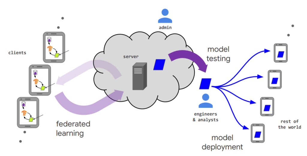
An answer is that knowledge on consumer units stays on consumer units, but
participates in coaching a worldwide mannequin. How? In so-called federated
studying(McMahan et al. 2016), there’s a central coordinator (“server”), in addition to
a probably enormous variety of shoppers (e.g., telephones) who take part in studying
on an “as-fits” foundation: e.g., if plugged in and on a high-speed connection.
At any time when they’re prepared to coach, shoppers are handed the present mannequin weights,
and carry out some variety of coaching iterations on their very own knowledge. They then ship
again gradient data to the server (extra on that quickly), whose job is to
replace the weights accordingly. Federated studying just isn’t the one conceivable
protocol to collectively prepare a deep studying mannequin whereas retaining the info personal:
A totally decentralized various might be gossip studying (Blot et al. 2016),
following the gossip protocol .
As of in the present day, nevertheless, I’m not conscious of present implementations in any of the
main deep studying frameworks.
In reality, even TensorFlow Federated (TFF), the library used on this submit, was
formally launched nearly a 12 months in the past. That means, all that is fairly new
know-how, someplace inbetween proof-of-concept state and manufacturing readiness.
So, let’s set expectations as to what you may get out of this submit.
What to anticipate from this submit
We begin with fast look at federated studying within the context of privateness
general. Subsequently, we introduce, by instance, a few of TFF’s fundamental constructing
blocks. Lastly, we present an entire picture classification instance utilizing Keras –
from R.
Whereas this appears like “enterprise as typical,” it’s not – or not fairly. With no R
bundle present, as of this writing, that will wrap TFF, we’re accessing its
performance utilizing $-syntax – not in itself an enormous downside. However there’s
one thing else.
TFF, whereas offering a Python API, itself just isn’t written in Python. As an alternative, it
is an inside language designed particularly for serializability and
distributed computation. One of many penalties is that TensorFlow (that’s: TF
versus TFF) code must be wrapped in calls to tf.operate, triggering
static-graph development. Nonetheless, as I write this, the TFF documentation
cautions:
“At the moment, TensorFlow doesn’t totally help serializing and deserializing
eager-mode TensorFlow.” Now once we name TFF from R, we add one other layer of
complexity, and usually tend to run into nook circumstances.
Subsequently, on the present
stage, when utilizing TFF from R it’s advisable to mess around with high-level
performance – utilizing Keras fashions – as an alternative of, e.g., translating to R the
low-level performance proven within the second TFF Core
tutorial.
One last comment earlier than we get began: As of this writing, there isn’t any
documentation on how you can really run federated coaching on “actual shoppers.” There’s, nevertheless, a
document
that describes how you can run TFF on Google Kubernetes Engine, and
deployment-related documentation is visibly and steadily rising.)
That stated, now how does federated studying relate to privateness, and the way does it
look in TFF?
Federated studying in context
In federated studying, consumer knowledge by no means leaves the gadget. So in a direct
sense, computations are personal. Nonetheless, gradient updates are despatched to a central
server, and that is the place privateness ensures could also be violated. In some circumstances, it
could also be simple to reconstruct the precise knowledge from the gradients – in an NLP process,
for instance, when the vocabulary is thought on the server, and gradient updates
are despatched for small items of textual content.
This may occasionally sound like a particular case, however basic strategies have been demonstrated
that work no matter circumstances. For instance, Zhu et
al. (Zhu, Liu, and Han 2019) use a “generative” strategy, with the server beginning
from randomly generated faux knowledge (leading to faux gradients) after which,
iteratively updating that knowledge to acquire gradients increasingly like the true
ones – at which level the true knowledge has been reconstructed.
Comparable assaults wouldn’t be possible have been gradients not despatched in clear textual content.
Nonetheless, the server wants to really use them to replace the mannequin – so it should
be capable of “see” them, proper? As hopeless as this sounds, there are methods out
of the dilemma. For instance, homomorphic
encryption, a way
that permits computation on encrypted knowledge. Or secure multi-party
aggregation,
usually achieved by way of secret
sharing, the place particular person items
of information (e.g.: particular person salaries) are break up up into “shares,” exchanged and
mixed with random knowledge in numerous methods, till lastly the specified international
consequence (e.g.: imply wage) is computed. (These are extraordinarily fascinating subjects
that sadly, by far surpass the scope of this submit.)
Now, with the server prevented from really “seeing” the gradients, an issue
nonetheless stays. The mannequin – particularly a high-capacity one, with many parameters
– might nonetheless memorize particular person coaching knowledge. Right here is the place differential
privateness comes into play. In differential privateness, noise is added to the
gradients to decouple them from precise coaching examples. (This
post
provides an introduction to differential privateness with TensorFlow, from R.)
As of this writing, TFF’s federal averaging mechanism (McMahan et al. 2016) doesn’t
but embody these further privacy-preserving methods. However analysis papers
exist that define algorithms for integrating each safe aggregation
(Bonawitz et al. 2016) and differential privateness (McMahan et al. 2017) .
Shopper-side and server-side computations
Like we stated above, at this level it’s advisable to primarily stick to
high-level computations utilizing TFF from R. (Presumably that’s what we’d be inquisitive about
in lots of circumstances, anyway.) Nevertheless it’s instructive to take a look at just a few constructing blocks
from a high-level, useful viewpoint.
In federated studying, mannequin coaching occurs on the shoppers. Shoppers every
compute their native gradients, in addition to native metrics. The server, then again,
calculates international gradient updates, in addition to international metrics.
Let’s say the metric is accuracy. Then shoppers and server each compute averages: native
averages and a worldwide common, respectively. All of the server might want to know to
decide the worldwide averages are the native ones and the respective pattern
sizes.
Let’s see how TFF would calculate a easy common.
The code on this submit was run with the present TensorFlow launch 2.1 and TFF
model 0.13.1. We use reticulate to put in and import TFF.
First, we’d like each consumer to have the ability to compute their very own native averages.
Here’s a operate that reduces an inventory of values to their sum and depend, each
on the identical time, after which returns their quotient.
The operate accommodates solely TensorFlow operations, not computations described in R
instantly; if there have been any, they must be wrapped in calls to
tf_function, calling for development of a static graph. (The identical would apply
to uncooked (non-TF) Python code.)
Now, this operate will nonetheless need to be wrapped (we’re attending to that in an
prompt), as TFF expects features that make use of TF operations to be
adorned by calls to tff$tf_computation. Earlier than we try this, one touch upon
the usage of dataset_reduce: Inside tff$tf_computation, the info that’s
handed in behaves like a dataset, so we are able to carry out tfdatasets operations
like dataset_map, dataset_filter and so on. on it.
Subsequent is the decision to tff$tf_computation we already alluded to, wrapping
get_local_temperature_average. We additionally want to point the
argument’s TFF-level kind.
(Within the context of this submit, TFF datatypes are
positively out-of-scope, however the TFF documentation has plenty of detailed
data in that regard. All we have to know proper now could be that we can go the info
as a listing.)
get_local_temperature_average <- tff$tf_computation(get_local_temperature_average, tff$SequenceType(tf$float32))Let’s take a look at this operate:
get_local_temperature_average(list(1, 2, 3))[1] 2In order that’s a neighborhood common, however we initially got down to compute a worldwide one.
Time to maneuver on to server aspect (code-wise).
Non-local computations are referred to as federated (not too surprisingly). Particular person
operations begin with federated_; and these need to be wrapped in
tff$federated_computation:
get_global_temperature_average <- operate(sensor_readings) {
  tff$federated_mean(tff$federated_map(get_local_temperature_average, sensor_readings))
}

get_global_temperature_average <- tff$federated_computation(
  get_global_temperature_average, tff$FederatedType(tff$SequenceType(tf$float32), tff$CLIENTS))
Calling this on an inventory of lists – every sub-list presumedly representing consumer knowledge – will show the worldwide (non-weighted) common:
[1] 7Now that we’ve gotten a little bit of a sense for “low-level TFF,” let’s prepare a
Keras mannequin the federated method.
Federated Keras
The setup for this instance appears to be like a bit extra Pythonian than typical. We’d like the
collections module from Python to utilize OrderedDicts, and we wish them to be handed to Python with out
intermediate conversion to R – that’s why we import the module with convert
set to FALSE.
For this instance, we use Kuzushiji-MNIST
(Clanuwat et al. 2018), which can conveniently be obtained by way of
tfds, the R wrapper for TensorFlow
Datasets.

TensorFlow datasets come as – properly – datasets, which usually could be simply
superb; right here nevertheless, we need to simulate totally different shoppers every with their very own
knowledge. The next code splits up the dataset into ten arbitrary – sequential,
for comfort – ranges and, for every vary (that’s: consumer), creates an inventory of
OrderedDicts which have the pictures as their x, and the labels as their y
part:
n_train <- 60000
n_test <- 10000

s <- seq(0, 90, by = 10)
train_ranges <- paste0("prepare[", s, "%:", s + 10, "%]") %>% as.list()
train_splits <- purrr::map(train_ranges, operate(r) tfds_load("kmnist", break up = r))

test_ranges <- paste0("take a look at[", s, "%:", s + 10, "%]") %>% as.list()
test_splits <- purrr::map(test_ranges, operate(r) tfds_load("kmnist", break up = r))

batch_size <- 100

create_client_dataset <- operate(supply, n_total, batch_size) {
  iter <- as_iterator(supply %>% dataset_batch(batch_size))
  output_sequence <- vector(mode = "listing", size = n_total/10/batch_size)
  i <- 1
  whereas (TRUE) {
    merchandise <- iter_next(iter)
    if (is.null(merchandise)) break
    x <- tf$reshape(tf$solid(merchandise$picture, tf$float32), list(100L,784L))/255
    y <- merchandise$label
    output_sequence[[i]] <-
      collections$OrderedDict("x" = np_array(x$numpy(), np$float32), "y" = y$numpy())
     i <- i + 1
  }
  output_sequence
}

federated_train_data <- purrr::map(
  train_splits, operate(break up) create_client_dataset(break up, n_train, batch_size))
As a fast verify, the next are the labels for the primary batch of photos for
consumer 5:
federated_train_data[[5]][[1]][['y']]> [0. 9. 8. 3. 1. 6. 2. 8. 8. 2. 5. 7. 1. 6. 1. 0. 3. 8. 5. 0. 5. 6. 6. 5.
2. 9. 5. 0. 3. 1. 0. 0. 6. 3. 6. 8. 2. 8. 9. 8. 5. 2. 9. 0. 2. 8. 7. 9.
2. 5. 1. 7. 1. 9. 1. 6. 0. 8. 6. 0. 5. 1. 3. 5. 4. 5. 3. 1. 3. 5. 3. 1.
0. 2. 7. 9. 6. 2. 8. 8. 4. 9. 4. 2. 9. 5. 7. 6. 5. 2. 0. 3. 4. 7. 8. 1.
8. 2. 7. 9.]The mannequin is a straightforward, one-layer sequential Keras mannequin. For TFF to have full
management over graph development, it must be outlined inside a operate. The
blueprint for creation is handed to tff$studying$from_keras_model, collectively
with a “dummy” batch that exemplifies how the coaching knowledge will look:
sample_batch = federated_train_data[[5]][[1]]

create_keras_model <- operate() {
  keras_model_sequential() %>%
    layer_dense(input_shape = 784,
                models = 10,
                kernel_initializer = "zeros",
                activation = "softmax")
}

model_fn <- operate() {
  keras_model <- create_keras_model()
  tff$studying$from_keras_model(
    keras_model,
    dummy_batch = sample_batch,
    loss = tf$keras$losses$SparseCategoricalCrossentropy(),
    metrics = list(tf$keras$metrics$SparseCategoricalAccuracy()))
}
Coaching is a stateful course of that retains updating mannequin weights (and if
relevant, optimizer states). It’s created through
tff$studying$build_federated_averaging_process …
iterative_process <- tff$studying$build_federated_averaging_process(
  model_fn,
  client_optimizer_fn = operate() tf$keras$optimizers$SGD(learning_rate = 0.02),
  server_optimizer_fn = operate() tf$keras$optimizers$SGD(learning_rate = 1.0))
… and on initialization, produces a beginning state:
state <- iterative_process$initialize()
state
<mannequin=<trainable=<[[0. 0. 0. ... 0. 0. 0.]
[0. 0. 0. ... 0. 0. 0.]
[0. 0. 0. ... 0. 0. 0.]
...
[0. 0. 0. ... 0. 0. 0.]
[0. 0. 0. ... 0. 0. 0.]
[0. 0. 0. ... 0. 0. 0.]],[0. 0. 0. 0. 0. 0. 0. 0. 0. 0.]>,non_trainable=<>>,optimizer_state=<0>,delta_aggregate_state=<>,model_broadcast_state=<>>Thus earlier than coaching, all of the state does is mirror our zero-initialized mannequin
weights.
Now, state transitions are achieved through calls to subsequent(). After one spherical
of coaching, the state then contains the “state correct” (weights, optimizer
parameters …) in addition to the present coaching metrics:
state_and_metrics <- iterative_process$`subsequent`(state, federated_train_data)

state <- state_and_metrics[0]
state
<mannequin=<trainable=<[[ 9.9695253e-06 -8.5083229e-05 -8.9266898e-05 ... -7.7834651e-05
-9.4819807e-05 3.4227365e-04]
[-5.4778640e-05 -1.5390900e-04 -1.7912561e-04 ... -1.4122366e-04
-2.4614178e-04 7.7663612e-04]
[-1.9177950e-04 -9.0706220e-05 -2.9841764e-04 ... -2.2249141e-04
-4.1685964e-04 1.1348884e-03]
...
[-1.3832574e-03 -5.3664664e-04 -3.6622395e-04 ... -9.0854493e-04
4.9618416e-04 2.6899918e-03]
[-7.7253254e-04 -2.4583895e-04 -8.3220737e-05 ... -4.5274393e-04
2.6396243e-04 1.7454443e-03]
[-2.4157032e-04 -1.3836231e-05 5.0371520e-05 ... -1.0652864e-04
1.5947431e-04 4.5250656e-04]],[-0.01264258 0.00974309 0.00814162 0.00846065 -0.0162328 0.01627758
-0.00445857 -0.01607843 0.00563046 0.00115899]>,non_trainable=<>>,optimizer_state=<1>,delta_aggregate_state=<>,model_broadcast_state=<>>metrics <- state_and_metrics[1]
metrics<sparse_categorical_accuracy=0.5710999965667725,loss=1.8662642240524292,keras_training_time_client_sum_sec=0.0>Let’s prepare for just a few extra epochs, retaining monitor of accuracy:
spherical:  2    accuracy:  0.6949
spherical:  3    accuracy:  0.7132
spherical:  4    accuracy:  0.7231
spherical:  5    accuracy:  0.7319
spherical:  6    accuracy:  0.7404
spherical:  7    accuracy:  0.7484
spherical:  8    accuracy:  0.7557
spherical:  9    accuracy:  0.7617
spherical:  10   accuracy:  0.7661
spherical:  11   accuracy:  0.7695
spherical:  12   accuracy:  0.7728
spherical:  13   accuracy:  0.7764
spherical:  14   accuracy:  0.7788
spherical:  15   accuracy:  0.7814
spherical:  16   accuracy:  0.7836
spherical:  17   accuracy:  0.7855
spherical:  18   accuracy:  0.7872
spherical:  19   accuracy:  0.7885
spherical:  20   accuracy:  0.7902
Coaching accuracy is rising constantly. These values characterize averages of
native accuracy measurements, so in the true world, they could properly be overly
optimistic (with every consumer overfitting on their respective knowledge). So
supplementing federated coaching, a federated analysis course of would wish to
be constructed so as to get a sensible view on efficiency. It is a matter to
come again to when extra associated TFF documentation is offered.
Conclusion
We hope you’ve loved this primary introduction to TFF utilizing R. Actually at this
time, it’s too early to be used in manufacturing; and for software in analysis (e.g., adversarial assaults on federated studying)
familiarity with “lowish”-level implementation code is required – regardless
whether or not you utilize R or Python.
Nonetheless, judging from exercise on GitHub, TFF is underneath very lively growth proper now (together with new documentation being added!), so we’re wanting ahead
to what’s to come back. Within the meantime, it’s by no means too early to start out studying the
ideas…
Thanks for studying!


