mannequin inversion assault by instance
How non-public are particular person knowledge within the context of machine studying fashions? The information used to coach the mannequin, say. There are
sorts of fashions the place the reply is easy. Take k-nearest-neighbors, for instance. There is just not even a mannequin with out the
full dataset. Or help vector machines. There isn’t any mannequin with out the help vectors. However neural networks? They’re simply
some composition of features, – no knowledge included.
The identical is true for knowledge fed to a deployed deep-learning mannequin. It’s fairly unlikely one might invert the ultimate softmax
output from a giant ResNet and get again the uncooked enter knowledge.
In principle, then, “hacking” an ordinary neural internet to spy on enter knowledge sounds illusory. In apply, nevertheless, there may be at all times
some real-world context. The context could also be different datasets, publicly out there, that may be linked to the “non-public” knowledge in
query. This can be a well-liked showcase utilized in advocating for differential privateness(Dwork et al. 2006): Take an “anonymized” dataset,
dig up complementary data from public sources, and de-anonymize information advert libitum. Some context in that sense will
typically be utilized in “black-box” assaults, ones that presuppose no insider details about the mannequin to be hacked.
However context will also be structural, equivalent to within the state of affairs demonstrated on this submit. For instance, assume a distributed
mannequin, the place units of layers run on completely different gadgets – embedded gadgets or cellphones, for instance. (A state of affairs like that
is typically seen as “white-box”(Wu et al. 2016), however in widespread understanding, white-box assaults in all probability presuppose some extra
insider information, equivalent to entry to mannequin structure and even, weights. I’d subsequently desire calling this white-ish at
most.) — Now assume that on this context, it’s potential to intercept, and work together with, a system that executes the deeper
layers of the mannequin. Primarily based on that system’s intermediate-level output, it’s potential to carry out mannequin inversion(Fredrikson et al. 2014),
that’s, to reconstruct the enter knowledge fed into the system.
On this submit, we’ll display such a mannequin inversion assault, principally porting the strategy given in a
notebook
discovered within the PySyft repository. We then experiment with completely different ranges of
(epsilon)-privacy, exploring affect on reconstruction success. This second half will make use of TensorFlow Privateness,
launched in a previous blog post.
Half 1: Mannequin inversion in motion
Instance dataset: All of the world’s letters
The general means of mannequin inversion used right here is the next. With no, or scarcely any, insider information a few mannequin,
– however given alternatives to repeatedly question it –, I need to learn to reconstruct unknown inputs based mostly on simply mannequin
outputs . Independently of authentic mannequin coaching, this, too, is a coaching course of; nevertheless, usually it won’t contain
the unique knowledge, as these gained’t be publicly out there. Nonetheless, for greatest success, the attacker mannequin is educated with knowledge as
comparable as potential to the unique coaching knowledge assumed. Pondering of photographs, for instance, and presupposing the favored view
of successive layers representing successively coarse-grained options, we wish that the surrogate knowledge to share as many
illustration areas with the true knowledge as potential – as much as the very highest layers earlier than closing classification, ideally.
If we wished to make use of classical MNIST for instance, one factor we might do is to solely use a number of the digits for coaching the
“actual” mannequin; and the remainder, for coaching the adversary. Let’s attempt one thing completely different although, one thing that may make the
enterprise tougher in addition to simpler on the similar time. Tougher, as a result of the dataset options exemplars extra complicated than MNIST
digits; simpler due to the identical cause: Extra might presumably be discovered, by the adversary, from a posh process.
Initially designed to develop a machine mannequin of idea studying and generalization (Lake, Salakhutdinov, and Tenenbaum 2015), the
OmniGlot dataset incorporates characters from fifty alphabets, break up into two
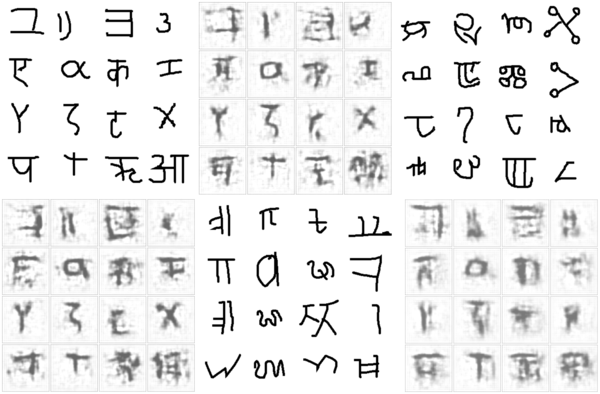
disjoint teams of thirty and twenty alphabets every. We’ll use the group of twenty to coach our goal mannequin. Here’s a
pattern:

Determine 1: Pattern from the twenty-alphabet set used to coach the goal mannequin (initially: ‘analysis set’)
The group of thirty we don’t use; as a substitute, we’ll make use of two small five-alphabet collections to coach the adversary and to check
reconstruction, respectively. (These small subsets of the unique “large” thirty-alphabet set are once more disjoint.)
Right here first is a pattern from the set used to coach the adversary.

Determine 2: Pattern from the five-alphabet set used to coach the adversary (initially: ‘background small 1’)
The opposite small subset can be used to check the adversary’s spying capabilities after coaching. Let’s peek at this one, too:

Determine 3: Pattern from the five-alphabet set used to check the adversary after coaching(initially: ‘background small 2’)
Conveniently, we will use tfds, the R wrapper to TensorFlow Datasets, to load these subsets:
Now first, we prepare the goal mannequin.
Practice goal mannequin
The dataset initially has 4 columns: the picture, of measurement 105 x 105; an alphabet id and a within-dataset character id; and a
label. For our use case, we’re probably not within the process the goal mannequin was/is used for; we simply need to get on the
knowledge. Mainly, no matter process we select, it’s not rather more than a dummy process. So, let’s simply say we prepare the goal to
classify characters by alphabet.
We thus throw out all unneeded options, maintaining simply the alphabet id and the picture itself:
# normalize and work with a single channel (photographs are black-and-white anyway)
preprocess_image <- operate(picture) {
  picture %>%
    tf$forged(dtype = tf$float32) %>%
    tf$truediv(y = 255) %>%
    tf$picture$rgb_to_grayscale()
}

# use the primary 11000 photographs for coaching
train_ds <- omni_train %>%
  dataset_take(11000) %>%
  dataset_map(operate(file) {
    file$picture <- preprocess_image(file$picture)
    list(file$picture, file$alphabet)}) %>%
  dataset_shuffle(1000) %>%
  dataset_batch(32)

# use the remaining 2180 information for validation
val_ds <- omni_train %>%
  dataset_skip(11000) %>%
  dataset_map(operate(file) {
    file$picture <- preprocess_image(file$picture)
    list(file$picture, file$alphabet)}) %>%
  dataset_batch(32)
The mannequin consists of two elements. The primary is imagined to run in a distributed trend; for instance, on cellular gadgets (stage
one). These gadgets then ship mannequin outputs to a central server, the place closing outcomes are computed (stage two). Certain, you’ll
be pondering, it is a handy setup for our state of affairs: If we intercept stage one outcomes, we – likely – achieve
entry to richer data than what’s contained in a mannequin’s closing output layer. — That’s right, however the state of affairs is
much less contrived than one may assume. Identical to federated studying (McMahan et al. 2016), it fulfills essential desiderata: Precise
coaching knowledge by no means leaves the gadgets, thus staying (in principle!) non-public; on the similar time, ingoing visitors to the server is
considerably decreased.
In our instance setup, the on-device mannequin is a convnet, whereas the server mannequin is an easy feedforward community.
We hyperlink each collectively as a TargetModel that when referred to as usually, will run each steps in succession. Nevertheless, we’ll give you the option
to name target_model$mobile_step() individually, thereby intercepting intermediate outcomes.
on_device_model <- keras_model_sequential() %>%
  layer_conv_2d(filters = 32, kernel_size = c(7, 7),
                input_shape = c(105, 105, 1), activation = "relu") %>%
  layer_batch_normalization() %>%
  layer_max_pooling_2d(pool_size = c(3, 3), strides = 3) %>%
  layer_dropout(0.2) %>%
  layer_conv_2d(filters = 32, kernel_size = c(7, 7), activation = "relu") %>%
  layer_batch_normalization() %>%
  layer_max_pooling_2d(pool_size = c(3, 3), strides = 2) %>%
  layer_dropout(0.2) %>%
  layer_conv_2d(filters = 32, kernel_size = c(5, 5), activation = "relu") %>%
  layer_batch_normalization() %>%
  layer_max_pooling_2d(pool_size = c(2, 2), strides = 2) %>%
  layer_dropout(0.2) %>%
  layer_conv_2d(filters = 32, kernel_size = c(3, 3), activation = "relu") %>%
  layer_batch_normalization() %>%
  layer_max_pooling_2d(pool_size = c(2, 2), strides = 2) %>%
  layer_dropout(0.2)

server_model <- keras_model_sequential() %>%
  layer_dense(models = 256, activation = "relu") %>%
  layer_flatten() %>%
  layer_dropout(0.2) %>%
  # we now have simply 20 completely different ids, however they don't seem to be in lexicographic order
  layer_dense(models = 50, activation = "softmax")

target_model <- operate() {
  keras_model_custom(title = "TargetModel", operate(self) {

    self$on_device_model <-on_device_model
    self$server_model <- server_model
    self$mobile_step <- operate(inputs)
      self$on_device_model(inputs)
    self$server_step <- operate(inputs)
      self$server_model(inputs)

    operate(inputs, masks = NULL) {
      inputs %>%
        self$mobile_step() %>%
        self$server_step()
    }
  })

}

mannequin <- target_model()
The general mannequin is a Keras customized mannequin, so we prepare it TensorFlow 2.x –
style. After ten epochs, coaching and validation accuracy are at ~0.84
and ~0.73, respectively – not dangerous in any respect for a 20-class discrimination process.
loss <- loss_sparse_categorical_crossentropy
optimizer <- optimizer_adam()

train_loss <- tf$keras$metrics$Imply(title='train_loss')
train_accuracy <-  tf$keras$metrics$SparseCategoricalAccuracy(title='train_accuracy')

val_loss <- tf$keras$metrics$Imply(title='val_loss')
val_accuracy <-  tf$keras$metrics$SparseCategoricalAccuracy(title='val_accuracy')

train_step <- operate(photographs, labels) {
  with (tf$GradientTape() %as% tape, {
    predictions <- mannequin(photographs)
    l <- loss(labels, predictions)
  })
  gradients <- tape$gradient(l, mannequin$trainable_variables)
  optimizer$apply_gradients(purrr::transpose(list(
    gradients, mannequin$trainable_variables
  )))
  train_loss(l)
  train_accuracy(labels, predictions)
}

val_step <- operate(photographs, labels) {
  predictions <- mannequin(photographs)
  l <- loss(labels, predictions)
  val_loss(l)
  val_accuracy(labels, predictions)
}


training_loop <- tf_function(autograph(operate(train_ds, val_ds) {
  for (b1 in train_ds) {
    train_step(b1[[1]], b1[[2]])
  }
  for (b2 in val_ds) {
    val_step(b2[[1]], b2[[2]])
  }

  tf$print("Practice accuracy", train_accuracy$outcome(),
           "    Validation Accuracy", val_accuracy$outcome())

  train_loss$reset_states()
  train_accuracy$reset_states()
  val_loss$reset_states()
  val_accuracy$reset_states()
}))


for (epoch in 1:10) {
  cat("Epoch: ", epoch, " -----------n")
  training_loop(train_ds, val_ds)
}
Epoch: 1 -----------
Practice accuracy 0.195090905 Validation Accuracy 0.376605511
Epoch: 2 -----------
Practice accuracy 0.472272724 Validation Accuracy 0.5243119
...
...
Epoch: 9 -----------
Practice accuracy 0.821454525 Validation Accuracy 0.720183492
Epoch: 10 -----------
Practice accuracy 0.840454519 Validation Accuracy 0.726605475Now, we prepare the adversary.
Practice adversary
The adversary’s common technique can be:
- Feed its small, surrogate dataset to the on-device mannequin. The output obtained might be thought to be a (extremely)
compressed model of the unique photographs. - Pass that “compressed” model as enter to its personal mannequin, which tries to reconstruct the unique photographs from the
sparse code. - Examine authentic photographs (these from the surrogate dataset) to the reconstruction pixel-wise. The purpose is to attenuate
the imply (squared, say) error.
Doesn’t this sound loads just like the decoding facet of an autoencoder? No surprise the attacker mannequin is a deconvolutional community.
Its enter – equivalently, the on-device mannequin’s output – is of measurement batch_size x 1 x 1 x 32. That’s, the knowledge is
encoded in 32 channels, however the spatial decision is 1. Identical to in an autoencoder working on photographs, we have to
upsample till we arrive on the authentic decision of 105 x 105.
That is precisely what’s occurring within the attacker mannequin:
attack_model <- operate() {

  keras_model_custom(title = "AttackModel", operate(self) {

    self$conv1 <-layer_conv_2d_transpose(filters = 32, kernel_size = 9,
                                         padding = "legitimate",
                                         strides = 1, activation = "relu")
    self$conv2 <- layer_conv_2d_transpose(filters = 32, kernel_size = 7,
                                          padding = "legitimate",
                                          strides = 2, activation = "relu")
    self$conv3 <- layer_conv_2d_transpose(filters = 1, kernel_size = 7,
                                          padding = "legitimate",
                                          strides = 2, activation = "relu")
    self$conv4 <- layer_conv_2d_transpose(filters = 1, kernel_size = 5,
                                          padding = "legitimate",
                                          strides = 2, activation = "relu")

    operate(inputs, masks = NULL) {
      inputs %>%
        # bs * 9 * 9 * 32
        # output = strides * (enter - 1) + kernel_size - 2 * padding
        self$conv1() %>%
        # bs * 23 * 23 * 32
        self$conv2() %>%
        # bs * 51 * 51 * 1
        self$conv3() %>%
        # bs * 105 * 105 * 1
        self$conv4()
    }
  })

}

attacker = attack_model()
To coach the adversary, we use one of many small (five-alphabet) subsets. To reiterate what was mentioned above, there isn’t a overlap
with the info used to coach the goal mannequin.
Right here, then, is the attacker coaching loop, striving to refine the decoding course of over 100 – quick – epochs:
attacker_criterion <- loss_mean_squared_error
attacker_optimizer <- optimizer_adam()
attacker_loss <- tf$keras$metrics$Imply(title='attacker_loss')
attacker_mse <-  tf$keras$metrics$MeanSquaredError(title='attacker_mse')

attacker_step <- operate(photographs) {

  attack_input <- mannequin$mobile_step(photographs)

  with (tf$GradientTape() %as% tape, {
    generated <- attacker(attack_input)
    l <- attacker_criterion(photographs, generated)
  })
  gradients <- tape$gradient(l, attacker$trainable_variables)
  attacker_optimizer$apply_gradients(purrr::transpose(list(
    gradients, attacker$trainable_variables
  )))
  attacker_loss(l)
  attacker_mse(photographs, generated)
}


attacker_training_loop <- tf_function(autograph(operate(attacker_ds) {
  for (b in attacker_ds) {
    attacker_step(b[[1]])
  }

  tf$print("mse: ", attacker_mse$outcome())

  attacker_loss$reset_states()
  attacker_mse$reset_states()
}))

for (epoch in 1:100) {
  cat("Epoch: ", epoch, " -----------n")
  attacker_training_loop(attacker_ds)
}
Epoch: 1 -----------
mse: 0.530902684
Epoch: 2 -----------
mse: 0.201351956
...
...
Epoch: 99 -----------
mse: 0.0413453057
Epoch: 100 -----------
mse: 0.0413028933The query now’s, – does it work? Has the attacker actually discovered to deduce precise knowledge from (stage one) mannequin output?
Check adversary
To check the adversary, we use the third dataset we downloaded, containing photographs from 5 yet-unseen alphabets. For show,
we choose simply the primary sixteen information – a totally arbitrary resolution, in fact.
test_ds <- omni_test %>%
  dataset_map(operate(file) {
    file$picture <- preprocess_image(file$picture)
    list(file$picture, file$alphabet)}) %>%
  dataset_take(16) %>%
  dataset_batch(16)

batch <- as_iterator(test_ds) %>% iterator_get_next()
photographs <- batch[[1]]

attack_input <- mannequin$mobile_step(photographs)
generated <- attacker(attack_input) %>% as.array()

generated[generated > 1] <- 1
generated <- generated[ , , , 1]
generated %>%
  purrr::array_tree(1) %>%
  purrr::map(as.raster) %>%
  purrr::iwalk(~{plot(.x)})
Identical to throughout the coaching course of, the adversary queries the goal mannequin (stage one), obtains the compressed
illustration, and makes an attempt to reconstruct the unique picture. (After all, in the true world, the setup could be completely different in
that the attacker would not have the ability to merely examine the pictures, as is the case right here. There would thus should be a way
to intercept, and make sense of, community visitors.)
To permit for simpler comparability (and enhance suspense …!), right here once more are the precise photographs, which we displayed already when
introducing the dataset:
Determine 4: First photographs from the take a look at set, the way in which they actually look.
And right here is the reconstruction:

Determine 5: First photographs from the take a look at set, as reconstructed by the adversary.
After all, it’s laborious to say how revealing these “guesses” are. There undoubtedly appears to be a connection to character
complexity; total, it looks as if the Greek and Roman letters, that are the least complicated, are additionally those most simply
reconstructed. Nonetheless, ultimately, how a lot privateness is misplaced will very a lot depend upon contextual elements.
At the beginning, do the exemplars within the dataset characterize people or courses of people? If – as in actuality
– the character X represents a category, it may not be so grave if we had been in a position to reconstruct “some X” right here: There are numerous
Xs within the dataset, all fairly comparable to one another; we’re unlikely to precisely to have reconstructed one particular, particular person
X. If, nevertheless, this was a dataset of particular person individuals, with all Xs being pictures of Alex, then in reconstructing an
X we now have successfully reconstructed Alex.
Second, in much less apparent eventualities, evaluating the diploma of privateness breach will doubtless surpass computation of quantitative
metrics, and contain the judgment of area specialists.
Talking of quantitative metrics although – our instance looks as if an ideal use case to experiment with differential
privateness. Differential privateness is measured by (epsilon) (decrease is healthier), the primary concept being that solutions to queries to a
system ought to rely as little as potential on the presence or absence of a single (any single) datapoint.
So, we are going to repeat the above experiment, utilizing TensorFlow Privateness (TFP) so as to add noise, in addition to clip gradients, throughout
optimization of the goal mannequin. We’ll attempt three completely different situations, leading to three completely different values for (epsilon)s,
and for every situation, examine the pictures reconstructed by the adversary.
Half 2: Differential privateness to the rescue
Sadly, the setup for this a part of the experiment requires somewhat workaround. Making use of the flexibleness afforded
by TensorFlow 2.x, our goal mannequin has been a customized mannequin, becoming a member of two distinct levels (“cellular” and “server”) that might be
referred to as independently.
TFP, nevertheless, does nonetheless not work with TensorFlow 2.x, that means we now have to make use of old-style, non-eager mannequin definitions and
coaching. Fortunately, the workaround can be straightforward.
First, load (and presumably, set up) libraries, taking care to disable TensorFlow V2 habits.
The coaching set is loaded, preprocessed and batched (almost) as earlier than.
omni_train <- tfds$load("omniglot", break up = "take a look at")

batch_size <- 32

train_ds <- omni_train %>%
  dataset_take(11000) %>%
  dataset_map(operate(file) {
    file$picture <- preprocess_image(file$picture)
    list(file$picture, file$alphabet)}) %>%
  dataset_shuffle(1000) %>%
  # want dataset_repeat() when not keen
  dataset_repeat() %>%
  dataset_batch(batch_size)
Practice goal mannequin – with TensorFlow Privateness
To coach the goal, we put the layers from each levels – “cellular” and “server” – into one sequential mannequin. Word how we
take away the dropout. It is because noise can be added throughout optimization anyway.
complete_model <- keras_model_sequential() %>%
  layer_conv_2d(filters = 32, kernel_size = c(7, 7),
                input_shape = c(105, 105, 1),
                activation = "relu") %>%
  layer_batch_normalization() %>%
  layer_max_pooling_2d(pool_size = c(3, 3), strides = 3) %>%
  #layer_dropout(0.2) %>%
  layer_conv_2d(filters = 32, kernel_size = c(7, 7), activation = "relu") %>%
  layer_batch_normalization() %>%
  layer_max_pooling_2d(pool_size = c(3, 3), strides = 2) %>%
  #layer_dropout(0.2) %>%
  layer_conv_2d(filters = 32, kernel_size = c(5, 5), activation = "relu") %>%
  layer_batch_normalization() %>%
  layer_max_pooling_2d(pool_size = c(2, 2), strides = 2) %>%
  #layer_dropout(0.2) %>%
  layer_conv_2d(filters = 32, kernel_size = c(3, 3), activation = "relu") %>%
  layer_batch_normalization() %>%
  layer_max_pooling_2d(pool_size = c(2, 2), strides = 2, title = "mobile_output") %>%
  #layer_dropout(0.2) %>%
  layer_dense(models = 256, activation = "relu") %>%
  layer_flatten() %>%
  #layer_dropout(0.2) %>%
  layer_dense(models = 50, activation = "softmax")
Utilizing TFP primarily means utilizing a TFP optimizer, one which clips gradients in keeping with some outlined magnitude and provides noise of
outlined measurement. noise_multiplier is the parameter we’re going to differ to reach at completely different (epsilon)s:
l2_norm_clip <- 1

# ratio of the usual deviation to the clipping norm
# we run coaching for every of the three values
noise_multiplier <- 0.7
noise_multiplier <- 0.5
noise_multiplier <- 0.3

# similar as batch measurement
num_microbatches <- k_cast(batch_size, "int32")
learning_rate <- 0.005

optimizer <- tfp$DPAdamGaussianOptimizer(
  l2_norm_clip = l2_norm_clip,
  noise_multiplier = noise_multiplier,
  num_microbatches = num_microbatches,
  learning_rate = learning_rate
)
In coaching the mannequin, the second essential change for TFP we have to make is to have loss and gradients computed on the
particular person stage.
# want so as to add noise to each particular person contribution
loss <- tf$keras$losses$SparseCategoricalCrossentropy(discount =   tf$keras$losses$Discount$NONE)

complete_model %>% compile(loss = loss, optimizer = optimizer, metrics = "sparse_categorical_accuracy")

num_epochs <- 20

n_train <- 13180

historical past <- complete_model %>% match(
  train_ds,
  # want steps_per_epoch when not in keen mode
  steps_per_epoch = n_train/batch_size,
  epochs = num_epochs)
To check three completely different (epsilon)s, we run this thrice, every time with a distinct noise_multiplier. Every time we arrive at
a distinct closing accuracy.
Here’s a synopsis, the place (epsilon) was computed like so:
compute_priv <- tfp$privateness$evaluation$compute_dp_sgd_privacy

compute_priv$compute_dp_sgd_privacy(
  # variety of information in coaching set
  n_train,
  batch_size,
  # noise_multiplier
  0.7, # or 0.5, or 0.3
  # variety of epochs
  20,
  # delta - shouldn't exceed 1/variety of examples in coaching set
1e-5)| 0.7 | 4.0 | 0.37 |
| 0.5 | 12.5 | 0.45 |
| 0.3 | 84.7 | 0.56 |
Now, because the adversary gained’t name the entire mannequin, we have to “reduce off” the second-stage layers. This leaves us with a mannequin
that executes stage-one logic solely. We save its weights, so we will later name it from the adversary:
intercepted <- keras_model(
  complete_model$enter,
  complete_model$get_layer("mobile_output")$output
)

intercepted %>% save_model_hdf5("./intercepted.hdf5")
Practice adversary (towards differentially non-public goal)
In coaching the adversary, we will hold a lot of the authentic code – that means, we’re again to TF-2 type. Even the definition of
the goal mannequin is similar as earlier than:
on_device_model <- keras_model_sequential() %>%
  [...]

server_model <- keras_model_sequential() %>%
  [...]

target_model <- function() {
  keras_model_custom(name = "TargetModel", function(self) {

    self$on_device_model <-on_device_model
    self$server_model <- server_model
    self$mobile_step <- function(inputs)
      self$on_device_model(inputs)
    self$server_step <- function(inputs)
      self$server_model(inputs)

    function(inputs, mask = NULL) {
      inputs %>%
        self$mobile_step() %>%
        self$server_step()
    }
  })
}

intercepted <- target_model()
But now, we load the trained target’s weights into the freshly defined model’s “mobile stage”:
intercepted$on_device_model$load_weights("intercepted.hdf5")And now, we’re back to the old training routine. Testing setup is the same as before, as well.
So how well does the adversary perform with differential privacy added to the picture?
Test adversary (against differentially private target)
Here, ordered by decreasing (epsilon), are the reconstructions. Again, we refrain from judging the results, for the same
reasons as before: In real-world applications, whether privacy is preserved “well enough” will depend on the context.
Here, first, are reconstructions from the run where the least noise was added.

Figure 6: Reconstruction attempts from a setup where the target model was trained with an epsilon of 84.7.
On to the next level of privacy protection:

Figure 7: Reconstruction attempts from a setup where the target model was trained with an epsilon of 12.5.
And the highest-(epsilon) one:

Figure 8: Reconstruction attempts from a setup where the target model was trained with an epsilon of 4.0.
Conclusion
Throughout this post, we’ve refrained from “over-commenting” on results, and focused on the why-and-how instead. This is
because in an artificial setup, chosen to facilitate exposition of concepts and methods, there really is no objective frame of
reference. What is a good reconstruction? What is a good (epsilon)? What constitutes a data breach? No-one knows.
In the real world, there is a context to everything – there are people involved, the people whose data we’re talking about.
There are organizations, regulations, laws. There are abstract principles, and there are implementations; different
implementations of the same “idea” can differ.
As in machine learning overall, research papers on privacy-, ethics- or otherwise society-related topics are full of LaTeX
formulae. Amid the math, let’s not forget the people.
Thanks for reading!
Fredrikson, Matthew, Eric Lantz, Somesh Jha, Simon Lin, David Web page, and Thomas Ristenpart. 2014. “Privateness in Pharmacogenetics: An Finish-to-Finish Case Research of Personalised Warfarin Dosing.” In Proceedings of the twenty third USENIX Convention on Safety Symposium, 17–32. SEC’14. USA: USENIX Affiliation.
Wu, X., M. Fredrikson, S. Jha, and J. F. Naughton. 2016. “A Methodology for Formalizing Mannequin-Inversion Assaults.” In 2016 IEEE twenty ninth Pc Safety Foundations Symposium (CSF), 355–70.


