Posit AI Weblog: Simple PixelCNN with tfprobability
We’ve seen fairly a couple of examples of unsupervised studying (or self-supervised studying, to decide on the extra appropriate however much less
standard time period) on this weblog.
Usually, these concerned Variational Autoencoders (VAEs), whose enchantment lies in them permitting to mannequin a latent area of
underlying, unbiased (ideally) components that decide the seen options. A attainable draw back will be the inferior
high quality of generated samples. Generative Adversarial Networks (GANs) are one other standard strategy. Conceptually, these are
extremely engaging on account of their game-theoretic framing. Nevertheless, they are often troublesome to coach. PixelCNN variants, on the
different hand – we’ll subsume all of them right here beneath PixelCNN – are typically recognized for his or her good outcomes. They appear to contain
some extra alchemy although. Beneath these circumstances, what could possibly be extra welcome than a simple method of experimenting with
them? By TensorFlow Likelihood (TFP) and its R wrapper, tfprobability, we now have
such a method.
This publish first provides an introduction to PixelCNN, concentrating on high-level ideas (leaving the main points for the curious
to look them up within the respective papers). We’ll then present an instance of utilizing tfprobability to experiment with the TFP
implementation.
PixelCNN ideas
Autoregressivity, or: We want (some) order
The fundamental thought in PixelCNN is autoregressivity. Every pixel is modeled as relying on all prior pixels. Formally:
[p(mathbf{x}) = prod_{i}p(x_i|x_0, x_1, …, x_{i-1})]
Now wait a second – what even are prior pixels? Final I noticed one photographs had been two-dimensional. So this implies now we have to impose
an order on the pixels. Generally this can be raster scan order: row after row, from left to proper. However when coping with
coloration photographs, there’s one thing else: At every place, we even have three depth values, one for every of pink, inexperienced,
and blue. The unique PixelCNN paper(Oord, Kalchbrenner, and Kavukcuoglu 2016) carried by autoregressivity right here as effectively, with a pixel’s depth for
pink relying on simply prior pixels, these for inexperienced relying on these similar prior pixels however moreover, the present worth
for pink, and people for blue relying on the prior pixels in addition to the present values for pink and inexperienced.
[p(x_i|mathbf{x}<i) = p(x_{i,R}|mathbf{x}<i) p(x_{i,G}|mathbf{x}<i, x_{i,R}) p(x_{i,B}|mathbf{x}<i, x_{i,R}, x_{i,G})]
Right here, the variant carried out in TFP, PixelCNN++(Salimans et al. 2017) , introduces a simplification; it factorizes the joint
distribution in a much less compute-intensive method.
Technically, then, we all know how autoregressivity is realized; intuitively, it could nonetheless appear shocking that imposing a raster
scan order “simply works” (to me, at the very least, it’s). Perhaps that is a type of factors the place compute energy efficiently
compensates for lack of an equal of a cognitive prior.
Masking, or: The place to not look
Now, PixelCNN ends in “CNN” for a purpose – as regular in picture processing, convolutional layers (or blocks thereof) are
concerned. However – is it not the very nature of a convolution that it computes a median of some kinds, wanting, for every
output pixel, not simply on the corresponding enter but additionally, at its spatial (or temporal) environment? How does that rhyme
with the look-at-just-prior-pixels technique?
Surprisingly, this drawback is simpler to unravel than it sounds. When making use of the convolutional kernel, simply multiply with a
masks that zeroes out any “forbidden pixels” – like on this instance for a 5×5 kernel, the place we’re about to compute the
convolved worth for row 3, column 3:
[left[begin{array}
{rrr}
1 & 1 & 1 & 1 & 1
1 & 1 & 1 & 1 & 1
1 & 1 & 1 & 0 & 0
0 & 0 & 0 & 0 & 0
0 & 0 & 0 & 0 & 0
end{array}right]
]
This makes the algorithm sincere, however introduces a special drawback: With every successive convolutional layer consuming its
predecessor’s output, there’s a repeatedly rising blind spot (so-called in analogy to the blind spot on the retina, however
positioned within the high proper) of pixels which might be by no means seen by the algorithm. Van den Oord et al. (2016)(Oord et al. 2016) repair this
by utilizing two completely different convolutional stacks, one continuing from high to backside, the opposite from left to proper.

Conditioning, or: Present me a kitten
To date, we’ve all the time talked about “producing photographs” in a purely generic method. However the true attraction lies in creating
samples of some specified kind – one of many lessons we’ve been coaching on, or orthogonal data fed into the community.
That is the place PixelCNN turns into Conditional PixelCNN(Oord et al. 2016), and additionally it is the place that feeling of magic resurfaces.
Once more, as “common math” it’s not exhausting to conceive. Right here, (mathbf{h}) is the extra enter we’re conditioning on:
[p(mathbf{x}| mathbf{h}) = prod_{i}p(x_i|x_0, x_1, …, x_{i-1}, mathbf{h})]
However how does this translate into neural community operations? It’s simply one other matrix multiplication ((V^T mathbf{h})) added
to the convolutional outputs ((W mathbf{x})).
[mathbf{y} = tanh(W_{k,f} mathbf{x} + V^T_{k,f} mathbf{h}) odot sigma(W_{k,g} mathbf{x} + V^T_{k,g} mathbf{h})]
(Should you’re questioning concerning the second half on the precise, after the Hadamard product signal – we received’t go into particulars, however in a
nutshell, it’s one other modification launched by (Oord et al. 2016), a switch of the “gating” precept from recurrent neural
networks, similar to GRUs and LSTMs, to the convolutional setting.)
So we see what goes into the choice of a pixel worth to pattern. However how is that call truly made?
Logistic combination probability , or: No pixel is an island
Once more, that is the place the TFP implementation doesn’t observe the unique paper, however the latter PixelCNN++ one. Initially,
pixels had been modeled as discrete values, selected by a softmax over 256 (0-255) attainable values. (That this truly labored
looks as if one other occasion of deep studying magic. Think about: On this mannequin, 254 is as removed from 255 as it’s from 0.)
In distinction, PixelCNN++ assumes an underlying steady distribution of coloration depth, and rounds to the closest integer.
That underlying distribution is a mix of logistic distributions, thus permitting for multimodality:
[nu sim sum_{i} pi_i logistic(mu_i, sigma_i)]
General structure and the PixelCNN distribution
General, PixelCNN++, as described in (Salimans et al. 2017), consists of six blocks. The blocks collectively make up a UNet-like
construction, successively downsizing the enter after which, upsampling once more:

In TFP’s PixelCNN distribution, the variety of blocks is configurable as num_hierarchies, the default being 3.
Every block consists of a customizable variety of layers, referred to as ResNet layers because of the residual connection (seen on the
proper) complementing the convolutional operations within the horizontal stack:

In TFP, the variety of these layers per block is configurable as num_resnet.
num_resnet and num_hierarchies are the parameters you’re most definitely to experiment with, however there are a couple of extra you possibly can
take a look at within the documentation. The variety of logistic
distributions within the combination can be configurable, however from my experiments it’s greatest to maintain that quantity somewhat low to keep away from
producing NaNs throughout coaching.
Let’s now see an entire instance.
Finish-to-end instance
Our playground can be QuickDraw, a dataset – nonetheless rising –
obtained by asking individuals to attract some object in at most twenty seconds, utilizing the mouse. (To see for your self, simply take a look at
the website). As of at the moment, there are greater than a fifty million cases, from 345
completely different lessons.
Before everything, these information had been chosen to take a break from MNIST and its variants. However similar to these (and lots of extra!),
QuickDraw will be obtained, in tfdatasets-ready type, by way of tfds, the R wrapper to
TensorFlow datasets. In distinction to the MNIST “household” although, the “actual samples” are themselves extremely irregular, and sometimes
even lacking important components. So to anchor judgment, when displaying generated samples we all the time present eight precise drawings
with them.
Making ready the information
The dataset being gigantic, we instruct tfds to load the primary 500,000 drawings “solely.”
To hurry up coaching additional, we then zoom in on twenty lessons. This successfully leaves us with ~ 1,100 – 1,500 drawings per
class.
# bee, bicycle, broccoli, butterfly, cactus,
# frog, guitar, lightning, penguin, pizza,
# rollerskates, sea turtle, sheep, snowflake, solar,
# swan, The Eiffel Tower, tractor, practice, tree
lessons <- c(26, 29, 43, 49, 50,
             125, 134, 172, 218, 225,
             246, 255, 258, 271, 295,
             296, 308, 320, 322, 323
)

classes_tensor <- tf$solid(lessons, tf$int64)

train_ds <- train_ds %>%
  dataset_filter(
    perform(document) tf$reduce_any(tf$equal(classes_tensor, document$label), -1L)
  )
The PixelCNN distribution expects values within the vary from 0 to 255 – no normalization required. Preprocessing then consists
of simply casting pixels and labels every to float:
preprocess <- perform(document) {
  document$picture <- tf$solid(document$picture, tf$float32)
  document$label <- tf$solid(document$label, tf$float32)
  list(tuple(document$picture, document$label))
}

batch_size <- 32

practice <- train_ds %>%
  dataset_map(preprocess) %>%
  dataset_shuffle(10000) %>%
  dataset_batch(batch_size)
Creating the mannequin
We now use tfd_pixel_cnn to outline what would be the
loglikelihood utilized by the mannequin.
dist <- tfd_pixel_cnn(
  image_shape = c(28, 28, 1),
  conditional_shape = list(),
  num_resnet = 5,
  num_hierarchies = 3,
  num_filters = 128,
  num_logistic_mix = 5,
  dropout_p =.5
)

image_input <- layer_input(form = c(28, 28, 1))
label_input <- layer_input(form = list())
log_prob <- dist %>% tfd_log_prob(image_input, conditional_input = label_input)
This practice loglikelihood is added as a loss to the mannequin, after which, the mannequin is compiled with simply an optimizer
specification solely. Throughout coaching, loss first decreased rapidly, however enhancements from later epochs had been smaller.
mannequin <- keras_model(inputs = list(image_input, label_input), outputs = log_prob)
mannequin$add_loss(-tf$reduce_mean(log_prob))
mannequin$compile(optimizer = optimizer_adam(lr = .001))

mannequin %>% match(practice, epochs = 10)
To collectively show actual and pretend photographs:
for (i in lessons) {
real_images <- train_ds %>%
dataset_filter(
perform(document) document$label == tf$solid(i, tf$int64)
) %>%
dataset_take(8) %>%
dataset_batch(8)
it <- as_iterator(real_images)
real_images <- iter_next(it)
real_images <- real_images$picture %>% as.array()
real_images <- real_images[ , , , 1]/255
generated_images <- dist %>% tfd_sample(8, conditional_input = i)
generated_images <- generated_images %>% as.array()
generated_images <- generated_images[ , , , 1]/255
photographs <- abind::abind(real_images, generated_images, alongside = 1)
png(paste0("draw_", i, ".png"), width = 8 * 28 * 10, peak = 2 * 28 * 10)
par(mfrow = c(2, 8), mar = c(0, 0, 0, 0))
photographs %>%
purrr::array_tree(1) %>%
purrr::map(as.raster) %>%
purrr::iwalk(plot)
dev.off()
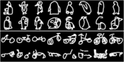
}From our twenty lessons, right here’s a alternative of six, every displaying actual drawings within the high row, and pretend ones under.


We most likely wouldn’t confuse the primary and second rows, however then, the precise human drawings exhibit monumental variation, too.
And nobody ever mentioned PixelCNN was an structure for idea studying. Be at liberty to mess around with different datasets of your
alternative – TFP’s PixelCNN distribution makes it straightforward.
Wrapping up
On this publish, we had tfprobability / TFP do all of the heavy lifting for us, and so, may concentrate on the underlying ideas.
Relying in your inclinations, this may be a perfect scenario – you don’t lose sight of the forest for the bushes. On the
different hand: Do you have to discover that altering the supplied parameters doesn’t obtain what you need, you might have a reference
implementation to start out from. So regardless of the consequence, the addition of such higher-level performance to TFP is a win for the
customers. (Should you’re a TFP developer studying this: Sure, we’d like extra :-)).
To everybody although, thanks for studying!
Salimans, Tim, Andrej Karpathy, Xi Chen, and Diederik P. Kingma. 2017. “PixelCNN++: A PixelCNN Implementation with Discretized Logistic Combination Probability and Different Modifications.” In ICLR.


