Deep Studying with R – KDnuggets – The Future of Work Institute

Picture from Bing Picture Creator

Who hasn’t been amused by technological developments significantly in artificial intelligence, from Alexa to Tesla self-driving vehicles and a myriad different improvements? I marvel on the developments each different day however what’s much more attention-grabbing is, if you get to have an thought of what underpins these improvements. Welcome to Artificial Intelligence and to the infinite potentialities of deep learning. In the event you’ve been questioning what it’s, you then’re dwelling.

On this tutorial, I’ll deconstruct the terminology and take you thru tips on how to carry out a deep studying process in R. To notice, this text will assume that you’ve got some fundamental understanding of machine learning ideas similar to regression, classification, and clustering.

Let’s begin with definitions of some terminologies surrounding the idea of deep studying:

Deep learning is a department of machine studying that teaches computer systems to imitate the cognitive features of the human mind. That is achieved via using synthetic neural networks that assist to unpack complicated patterns in knowledge units. With deep studying, a pc can classify sounds, photographs, and even texts.

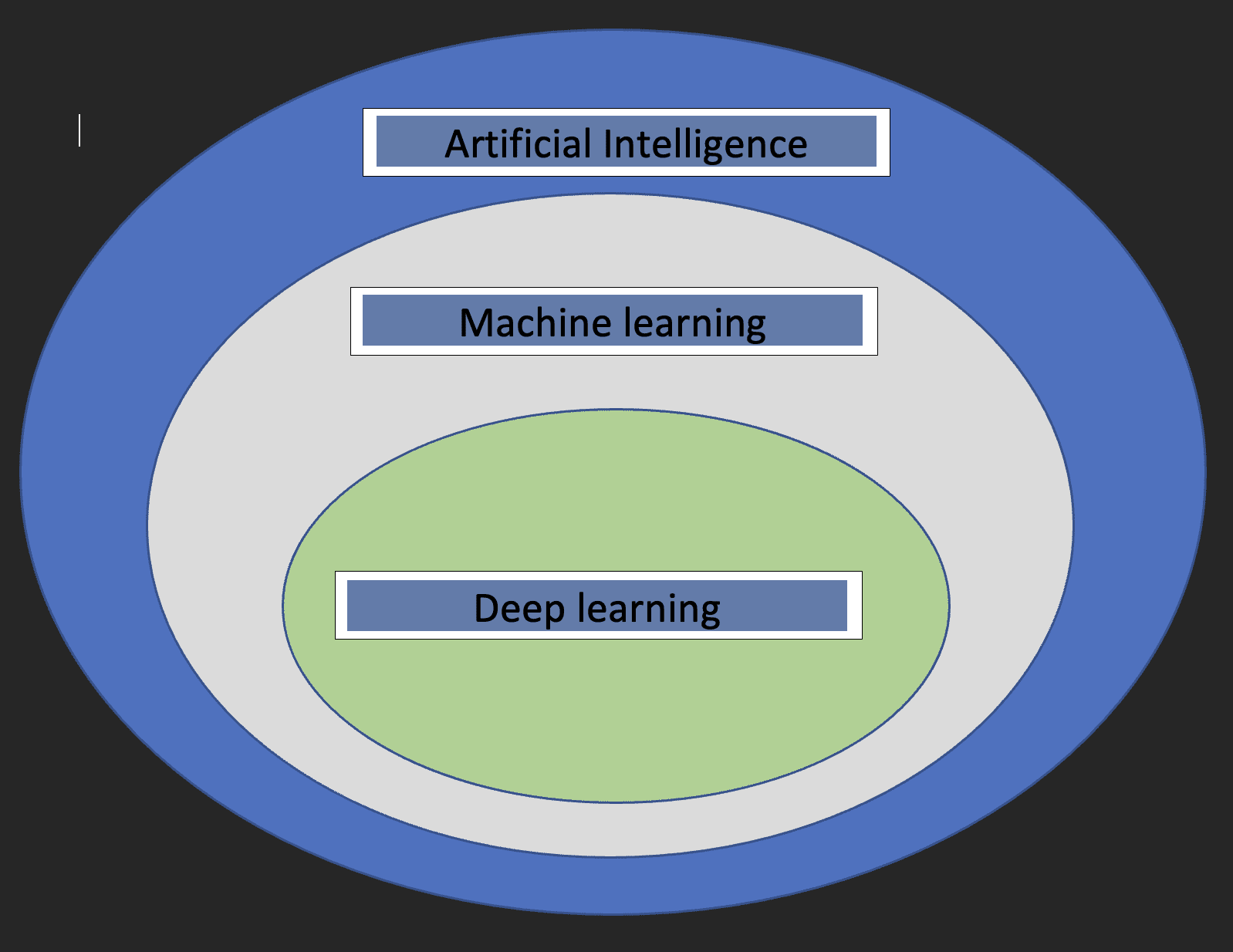
Earlier than we dive into the specifics of Deep studying, it might be good to grasp what machine studying and synthetic intelligence are and the way the three ideas relate to one another.

Artificial intelligence: It is a department of pc science that’s involved with the event of machines whose functioning mimics the human mind.

Machine studying: It is a subset of Synthetic Intelligence that allows computer systems to study from knowledge.

With the above definitions, we now have an thought of how deep studying pertains to synthetic intelligence and machine studying.

The diagram beneath will assist present the connection.

Two essential issues to notice about deep studying are:

Requires large volumes of knowledge
Requires high-performance computing energy

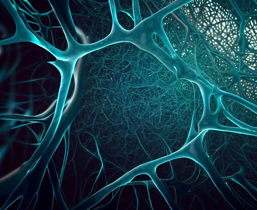
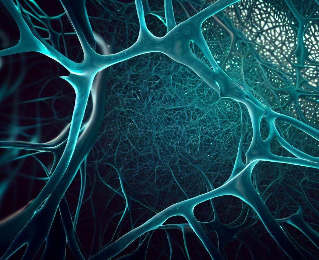
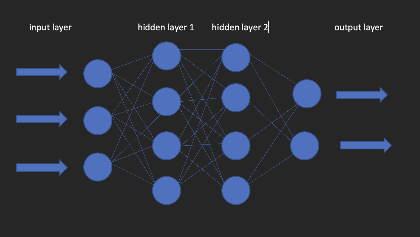
These are the constructing blocks of deep studying fashions. Because the identify suggests, the phrase neural comes from neurons, similar to the neurons of the human mind. Truly, the structure of deep neural networks will get its inspiration from the construction of the human mind.

A neural community has an enter layer, one hidden layer and an output layer. This community is named a shallow neural community. When we’ve a couple of hidden layer, it turns into a deep neural community, the place the layers could possibly be as many as 100’s.

The picture beneath exhibits what a neural community appears to be like like.

This brings us to the query of tips on how to construct deep studying fashions in R? Enter kera!

Keras is an open-source deep studying library that makes it straightforward to make use of neural networks in machine studying. This library is a wrapper that makes use of TensorFlow as a backend engine. Nevertheless, there are different choices for the backend similar to Theano or CNTK.

Allow us to now set up each TensorFlow and Keras.

Begin with making a digital setting utilizing reticulate

library(reticulate)
virtualenv_create("virtualenv", python = "/path/to/your/python3")

set up.packages(“tensorflow”) #That is solely achieved as soon as!

library(tensorflow)

install_tensorflow(envname = "/path/to/your/virtualenv", model = "cpu")

set up.packages(“keras”) #do that as soon as!

library(keras)

install_keras(envname = "/path/to/your/virtualenv")

# verify the set up was profitable
tf$fixed("Hiya TensorFlow!")

Now that our configurations are set, we will head over to how we will use deep studying to unravel a classification drawback.

The information I’ll use for this tutorial is from an ongoing Wage Survey achieved by https://www.askamanager.org.

The primary query requested within the type is how a lot cash do you make, plus a few extra particulars similar to business, age, years of expertise, and so on. The small print are collected right into a Google sheet from which I obtained the information.

The issue we wish to clear up with knowledge is to have the ability to give you a deep studying mannequin that predicts how a lot somebody may doubtlessly earn given data similar to age, gender, years of expertise, and highest stage of schooling.

Load the libraries that we’ll require.

library(dplyr)
library(keras)
library(caTools)

Import the information

url <- “https://uncooked.githubusercontent.com/oyogo/salary_dashboard/grasp/knowledge/salary_data_cleaned.csv”

salary_data <- learn.csv(url)

Choose the columns that we’d like

salary_data <- salary_data %>% choose(age,professional_experience_years,gender,highest_edu_level,annual_salary)

Keep in mind the pc science GIGO idea? (Rubbish in Rubbish Out). Properly, this idea is completely relevant right here as it’s in different domains. The outcomes of our coaching will largely depend upon the standard of the information we use. That is what brings knowledge cleansing and transformation, a vital step in any Data Science undertaking.

A few of the key points knowledge cleansing seeks to handle are; consistency, lacking values, spelling points, outliers, and knowledge varieties. I received’t go into the small print on how these points are tackled and that is for the straightforward motive of not eager to digress from the subject material of this text. Due to this fact, I’ll use the cleaned model of the information however when you’re keen on figuring out how the cleansing bit was dealt with, test this text out.

Synthetic neural networks settle for numeric variables solely and seeing that a few of our variables are of categorical nature, we might want to encode such into numbers. That is what varieties a part of the data preprocessing step, which is important as a result of as a rule, you received’t get knowledge that’s prepared for modeling.

# create an encoder perform
encode_ordinal <- perform(x, order = distinctive(x)) {
  x <- as.numeric(issue(x, ranges = order, exclude = NULL))
}

salary_data <- salary_data %>% mutate(
  highest_edu_level = encode_ordinal(highest_edu_level, order = c("Excessive Faculty","School diploma","Grasp's diploma","Skilled diploma (MD, JD, and so on.)","PhD")),
  professional_experience_years = encode_ordinal(professional_experience_years, 
  order = c("1 yr or much less", "2 - 4 years","5-7 years",  "8 - 10 years", "11 - 20 years", "21 - 30 years", "31 - 40 years", "41 years or extra")),
  age = encode_ordinal(age, order = c( "beneath 18", "18-24","25-34", "35-44", "45-54", "55-64","65 or over")),
  gender = case_when(gender== "Girl" ~ 0,
                 	gender == "Man" ~ 1))

Seeing that we wish to clear up a classification, we have to categorize the annual wage into two courses in order that we use it because the response variable.

salary_data <- salary_data %>%
  mutate(classes = case_when(
	annual_salary <= 100000 ~ 0,
	annual_salary > 100000 ~ 1))

salary_data <- salary_data %>% choose(-annual_salary)

As within the fundamental machine studying approaches; regression, classification, and clustering, we might want to break up our knowledge into coaching and testing units. We do that utilizing the 80-20 guidelines, which is 80% of the dataset for coaching and 20% for testing. This isn’t solid on stones, as you’ll be able to resolve to make use of any break up ratios as you see match, however understand that the coaching set ought to have share of the odds.

set.seed(123)

sample_split <- pattern.break up(Y = salary_data$classes, SplitRatio = 0.7)
train_set <- subset(x=salary_data, sample_split == TRUE)
test_set <- subset(x = salary_data, sample_split == FALSE)

y_train <- train_set$classes
y_test <- test_set$classes
x_train <- train_set %>% choose(-categories)
x_test <- test_set %>% choose(-categories)

Keras takes in inputs within the type of matrices or arrays. We use the as.matrix perform for the conversion. Additionally, we have to scale the predictor variables after which we convert the response variable to categorical knowledge kind.

x <- as.matrix(apply(x_train, 2, perform(x) (x-min(x))/(max(x) - min(x))))

y <- to_categorical(y_train, num_classes = 2)

Instantiate the mannequin

Create a sequential mannequin onto which we’ll add layers utilizing the pipe operator.

mannequin = keras_model_sequential()

Configure the Layers

The input_shape specifies the form of the enter knowledge. In our case, we’ve obtained that utilizing the ncol perform. activation: Right here we specify the activation perform; a mathematical perform that transforms the output to a desired non-linear format earlier than passing it to the subsequent layer.

models: the variety of neurons in every layer of the neural community.

mannequin %>%
  layer_dense(input_shape = ncol(x), models = 10, activation = "relu") %>%
  layer_dense(models = 10, activation = "relu") %>%
  layer_dense(models = 2, activation = "sigmoid")

We use the compile technique to do that. The perform takes three arguments;

optimizer : This object specifies the coaching process. loss : That is the perform to reduce throughout optimization. Choices out there are mse (imply sq. error), binary_crossentropy and categorical_crossentropy.

metrics : What we use to watch the coaching. Accuracy for classification issues.

mannequin %>%
  compile(
	loss = "binary_crossentropy",
	optimizer = "adagrad",
	metrics = "accuracy"
)

We are able to now match the mannequin utilizing the match technique from Keras. A few of the arguments that match takes in are:

epochs : An epoch is an iteration over the coaching dataset.

batch_size : The mannequin slices the matrix/array handed to it into smaller batches over which it iterates throughout coaching.

validation_split : Keras might want to slice a portion of the coaching knowledge to acquire a validation set that can be used to judge mannequin efficiency for every epoch.

shuffle : Right here you Point out whether or not you wish to shuffle your coaching knowledge earlier than every epoch.

match = mannequin %>%
  match(
	x = x,
	y = y,
	shuffle = T,
	validation_split = 0.2,
	epochs = 100,
	batch_size = 5
)

Consider the mannequin

To acquire the accuracy worth of the mannequin use the consider perform as beneath.

y_test <- to_categorical(y_test, num_classes = 2)
mannequin %>% consider(as.matrix(x_test),y_test)

Prediction

To foretell on new knowledge use the predict_classes perform from keras library as beneath.

mannequin %>% predict(as.matrix(x_test))

This text has taken you thru the fundamentals of deep studying with Keras in R. You’re welcome to dive deeper for higher understanding, mess around with the parameters, get your arms soiled with knowledge preparation, and maybe scale the computations by leveraging the ability of cloud computing.

Clinton Oyogo author at Saturn Cloud believes that analyzing knowledge for actionable insights is a vital a part of his day-to-day work. Along with his expertise in knowledge visualization, knowledge wrangling, and machine studying, he takes delight in his work as a knowledge scientist.

Original. Reposted with permission.