Posit AI Weblog: Practice in R, run on Android: Picture segmentation with torch

In a way, picture segmentation is just not that completely different from picture classification. It’s simply that as a substitute of categorizing a picture as a complete, segmentation leads to a label for each single pixel. And as in picture classification, the classes of curiosity rely on the duty: Foreground versus background, say; several types of tissue; several types of vegetation; et cetera.

The current submit is just not the primary on this weblog to deal with that subject; and like all prior ones, it makes use of a U-Web structure to realize its purpose. Central traits (of this submit, not U-Web) are:

1. It demonstrates the best way to carry out information augmentation for a picture segmentation activity.

2. It makes use of luz, torch’s high-level interface, to coach the mannequin.

3. It JIT-traces the skilled mannequin and saves it for deployment on cellular units. (JIT being the acronym generally used for the torch just-in-time compiler.)

4. It contains proof-of-concept code (although not a dialogue) of the saved mannequin being run on Android.

And if you happen to suppose that this in itself is just not thrilling sufficient – our activity right here is to seek out cats and canines. What might be extra useful than a cellular utility ensuring you may distinguish your cat from the fluffy couch she’s reposing on?

Practice in R

We begin by making ready the info.

Pre-processing and information augmentation

As offered by torchdatasets, the Oxford Pet Dataset comes with three variants of goal information to select from: the general class (cat or canine), the person breed (there are thirty-seven of them), and a pixel-level segmentation with three classes: foreground, boundary, and background. The latter is the default; and it’s precisely the kind of goal we want.

A name to oxford_pet_dataset(root = dir) will set off the preliminary obtain:

# want torch > 0.6.1
# might must run remotes::install_github("mlverse/torch", ref = remotes::github_pull("713")) relying on while you learn this
library(torch) 
library(torchvision)
library(torchdatasets)
library(luz)

dir <- "~/.torch-datasets/oxford_pet_dataset"

ds <- oxford_pet_dataset(root = dir)

Photographs (and corresponding masks) come in numerous sizes. For coaching, nevertheless, we’ll want all of them to be the identical measurement. This may be achieved by passing in remodel = and target_transform = arguments. However what about information augmentation (mainly at all times a helpful measure to take)? Think about we make use of random flipping. An enter picture will likely be flipped – or not – based on some chance. But when the picture is flipped, the masks higher had be, as properly! Enter and goal transformations aren’t unbiased, on this case.

An answer is to create a wrapper round oxford_pet_dataset() that lets us “hook into” the .getitem() technique, like so:

pet_dataset <- torch::dataset(
  
  inherit = oxford_pet_dataset,
  
  initialize = perform(..., measurement, normalize = TRUE, augmentation = NULL) {
    
    self$augmentation <- augmentation
    
    input_transform <- perform(x) {
      x <- x %>%
        transform_to_tensor() %>%
        transform_resize(measurement) 
      # we'll make use of pre-trained MobileNet v2 as a characteristic extractor
      # => normalize so as to match the distribution of photographs it was skilled with
      if (isTRUE(normalize)) x <- x %>%
        transform_normalize(imply = c(0.485, 0.456, 0.406),
                            std = c(0.229, 0.224, 0.225))
      x
    }
    
    target_transform <- perform(x) {
      x <- torch_tensor(x, dtype = torch_long())
      x <- x[newaxis,..]
      # interpolation = 0 makes certain we nonetheless find yourself with integer lessons
      x <- transform_resize(x, measurement, interpolation = 0)
    }
    
    tremendous$initialize(
      ...,
      remodel = input_transform,
      target_transform = target_transform
    )
    
  },
  .getitem = perform(i) {
    
    merchandise <- tremendous$.getitem(i)
    if (!is.null(self$augmentation)) 
      self$augmentation(merchandise)
    else
      list(x = merchandise$x, y = merchandise$y[1,..])
  }
)

All we now have to do now’s create a customized perform that lets us determine on what augmentation to use to every input-target pair, after which, manually name the respective transformation capabilities.

Right here, we flip, on common, each second picture, and if we do, we flip the masks as properly. The second transformation – orchestrating random modifications in brightness, saturation, and distinction – is utilized to the enter picture solely.

augmentation <- perform(merchandise) {
  
  vflip <- runif(1) > 0.5
  
  x <- merchandise$x
  y <- merchandise$y
  
  if (isTRUE(vflip)) {
    x <- transform_vflip(x)
    y <- transform_vflip(y)
  }
  
  x <- transform_color_jitter(x, brightness = 0.5, saturation = 0.3, distinction = 0.3)
  
  list(x = x, y = y[1,..])
  
}

We now make use of the wrapper, pet_dataset(), to instantiate the coaching and validation units, and create the respective information loaders.

train_ds <- pet_dataset(root = dir,
                        cut up = "practice",
                        measurement = c(224, 224),
                        augmentation = augmentation)
valid_ds <- pet_dataset(root = dir,
                        cut up = "legitimate",
                        measurement = c(224, 224))

train_dl <- dataloader(train_ds, batch_size = 32, shuffle = TRUE)
valid_dl <- dataloader(valid_ds, batch_size = 32)

Mannequin definition

The mannequin implements a traditional U-Web structure, with an encoding stage (the “down” cross), a decoding stage (the “up” cross), and importantly, a “bridge” that passes options preserved from the encoding stage on to corresponding layers within the decoding stage.

Encoder

First, we now have the encoder. It makes use of a pre-trained mannequin (MobileNet v2) as its characteristic extractor.

The encoder splits up MobileNet v2’s characteristic extraction blocks into a number of phases, and applies one stage after the opposite. Respective outcomes are saved in an inventory.

encoder <- nn_module(
  
  initialize = perform() {
    mannequin <- model_mobilenet_v2(pretrained = TRUE)
    self$phases <- nn_module_list(list(
      nn_identity(),
      mannequin$options[1:2],
      mannequin$options[3:4],
      mannequin$options[5:7],
      mannequin$options[8:14],
      mannequin$options[15:18]
    ))

    for (par in self$parameters) {
      par$requires_grad_(FALSE)
    }

  },
  ahead = perform(x) {
    options <- list()
    for (i in 1:length(self$phases)) {
      x <- self$phases[[i]](x)
      options[[length(features) + 1]] <- x
    }
    options
  }
)

Decoder

The decoder is made up of configurable blocks. A block receives two enter tensors: one that’s the results of making use of the earlier decoder block, and one which holds the characteristic map produced within the matching encoder stage. Within the ahead cross, first the previous is upsampled, and handed by way of a nonlinearity. The intermediate result’s then prepended to the second argument, the channeled-through characteristic map. On the resultant tensor, a convolution is utilized, adopted by one other nonlinearity.

decoder_block <- nn_module(
  
  initialize = perform(in_channels, skip_channels, out_channels) {
    self$upsample <- nn_conv_transpose2d(
      in_channels = in_channels,
      out_channels = out_channels,
      kernel_size = 2,
      stride = 2
    )
    self$activation <- nn_relu()
    self$conv <- nn_conv2d(
      in_channels = out_channels + skip_channels,
      out_channels = out_channels,
      kernel_size = 3,
      padding = "similar"
    )
  },
  ahead = perform(x, skip) {
    x <- x %>%
      self$upsample() %>%
      self$activation()

    enter <- torch_cat(list(x, skip), dim = 2)

    enter %>%
      self$conv() %>%
      self$activation()
  }
)

The decoder itself “simply” instantiates and runs by way of the blocks:

decoder <- nn_module(
  
  initialize = perform(
    decoder_channels = c(256, 128, 64, 32, 16),
    encoder_channels = c(16, 24, 32, 96, 320)
  ) {

    encoder_channels <- rev(encoder_channels)
    skip_channels <- c(encoder_channels[-1], 3)
    in_channels <- c(encoder_channels[1], decoder_channels)

    depth <- length(encoder_channels)

    self$blocks <- nn_module_list()
    for (i in seq_len(depth)) {
      self$blocks$append(decoder_block(
        in_channels = in_channels[i],
        skip_channels = skip_channels[i],
        out_channels = decoder_channels[i]
      ))
    }

  },
  ahead = perform(options) {
    options <- rev(options)
    x <- options[[1]]
    for (i in seq_along(self$blocks)) {
      x <- self$blocks[[i]](x, options[[i+1]])
    }
    x
  }
)

Prime-level module

Lastly, the top-level module generates the category rating. In our activity, there are three pixel lessons. The score-producing submodule can then simply be a remaining convolution, producing three channels:

mannequin <- nn_module(
  
  initialize = perform() {
    self$encoder <- encoder()
    self$decoder <- decoder()
    self$output <- nn_sequential(
      nn_conv2d(in_channels = 16,
                out_channels = 3,
                kernel_size = 3,
                padding = "similar")
    )
  },
  ahead = perform(x) {
    x %>%
      self$encoder() %>%
      self$decoder() %>%
      self$output()
  }
)

Mannequin coaching and (visible) analysis

With luz, mannequin coaching is a matter of two verbs, setup() and match(). The educational fee has been decided, for this particular case, utilizing luz::lr_finder(); you’ll doubtless have to alter it when experimenting with completely different types of information augmentation (and completely different information units).

mannequin <- mannequin %>%
  setup(optimizer = optim_adam, loss = nn_cross_entropy_loss())

fitted <- mannequin %>%
  set_opt_hparams(lr = 1e-3) %>%
  match(train_dl, epochs = 10, valid_data = valid_dl)

Right here is an excerpt of how coaching efficiency developed in my case:

# Epoch 1/10
# Practice metrics: Loss: 0.504                                                           
# Legitimate metrics: Loss: 0.3154

# Epoch 2/10
# Practice metrics: Loss: 0.2845                                                           
# Legitimate metrics: Loss: 0.2549

...
...

# Epoch 9/10
# Practice metrics: Loss: 0.1368                                                           
# Legitimate metrics: Loss: 0.2332

# Epoch 10/10
# Practice metrics: Loss: 0.1299                                                           
# Legitimate metrics: Loss: 0.2511

Numbers are simply numbers – how good is the skilled mannequin actually at segmenting pet photographs? To seek out out, we generate segmentation masks for the primary eight observations within the validation set, and plot them overlaid on the photographs. A handy method to plot a picture and superimpose a masks is offered by the raster package deal.

Pixel intensities must be between zero and one, which is why within the dataset wrapper, we now have made it so normalization could be switched off. To plot the precise photographs, we simply instantiate a clone of valid_ds that leaves the pixel values unchanged. (The predictions, alternatively, will nonetheless must be obtained from the unique validation set.)

valid_ds_4plot <- pet_dataset(
  root = dir,
  cut up = "legitimate",
  measurement = c(224, 224),
  normalize = FALSE
)

Lastly, the predictions are generated in a loop, and overlaid over the photographs one-by-one:

indices <- 1:8

preds <- predict(fitted, dataloader(dataset_subset(valid_ds, indices)))

png("pet_segmentation.png", width = 1200, top = 600, bg = "black")

par(mfcol = c(2, 4), mar = rep(2, 4))

for (i in indices) {
  
  masks <- as.array(torch_argmax(preds[i,..], 1)$to(machine = "cpu"))
  masks <- raster::ratify(raster::raster(masks))
  
  img <- as.array(valid_ds_4plot[i][[1]]$permute(c(2,3,1)))
  cond <- img > 0.99999
  img[cond] <- 0.99999
  img <- raster::brick(img)
  
  # plot picture
  raster::plotRGB(img, scale = 1, asp = 1, margins = TRUE)
  # overlay masks
  plot(masks, alpha = 0.4, legend = FALSE, axes = FALSE, add = TRUE)
  
}

Now onto operating this mannequin “within the wild” (properly, type of).

JIT-trace and run on Android

Tracing the skilled mannequin will convert it to a kind that may be loaded in R-less environments – for instance, from Python, C++, or Java.

We entry the torch mannequin underlying the fitted luz object, and hint it – the place tracing means calling it as soon as, on a pattern commentary:

m <- fitted$mannequin
x <- coro::accumulate(train_dl, 1)

traced <- jit_trace(m, x[[1]]$x)

The traced mannequin might now be saved to be used with Python or C++, like so:

traced %>% jit_save("traced_model.pt")

Nevertheless, since we already know we’d prefer to deploy it on Android, we as a substitute make use of the specialised perform jit_save_for_mobile() that, moreover, generates bytecode:

# want torch > 0.6.1
jit_save_for_mobile(traced_model, "model_bytecode.pt")

And that’s it for the R facet!

For operating on Android, I made heavy use of PyTorch Cell’s Android example apps, particularly the image segmentation one.

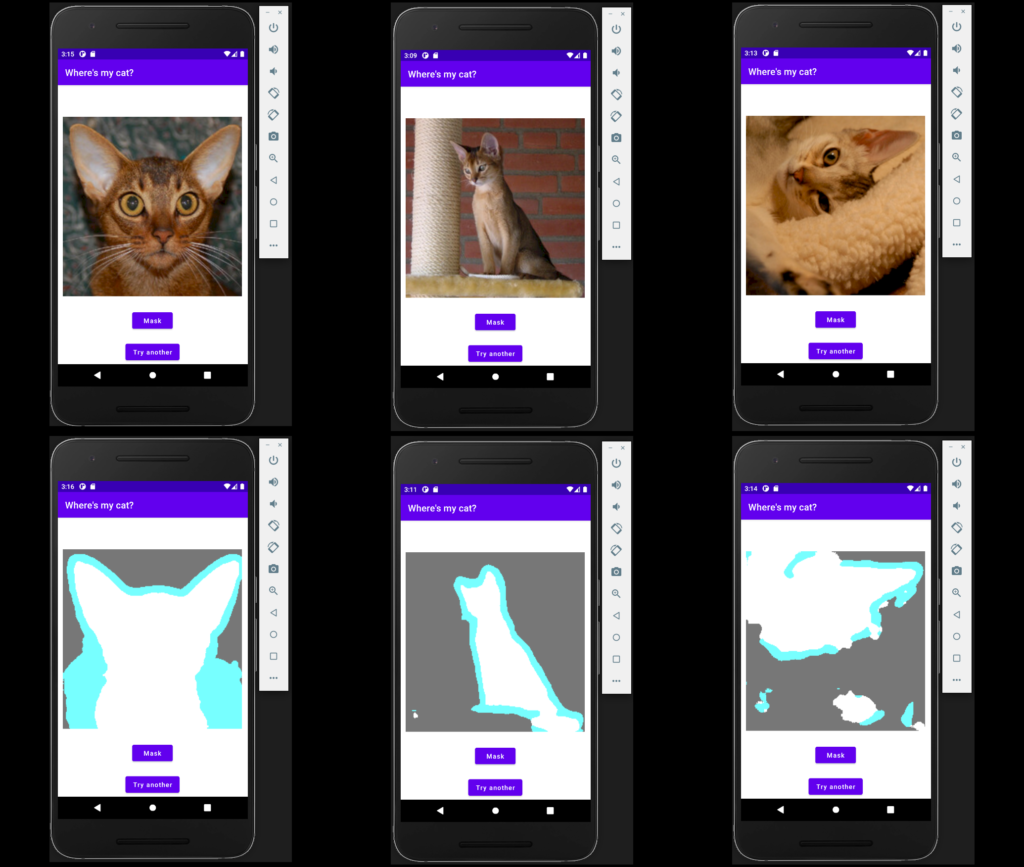
The precise proof-of-concept code for this submit (which was used to generate the under image) could also be discovered right here: https://github.com/skeydan/ImageSegmentation. (Be warned although – it’s my first Android utility!).

In fact, we nonetheless must attempt to discover the cat. Right here is the mannequin, run on a tool emulator in Android Studio, on three photographs (from the Oxford Pet Dataset) chosen for, firstly, a variety in problem, and secondly, properly … for cuteness:

Thanks for studying!