Posit AI Weblog: Group highlight: Enjoyable with torchopt

From the start, it has been thrilling to look at the rising variety of packages growing within the torch ecosystem. What’s wonderful is the number of issues folks do with torch: prolong its performance; combine and put to domain-specific use its low-level automated differentiation infrastructure; port neural community architectures … and final however not least, reply scientific questions.

This weblog submit will introduce, briefly and moderately subjective kind, considered one of these packages: torchopt. Earlier than we begin, one factor we must always most likely say much more typically: In case you’d prefer to publish a submit on this weblog, on the bundle you’re growing or the best way you utilize R-language deep studying frameworks, tell us – you’re greater than welcome!

torchopt

torchopt is a bundle developed by Gilberto Camara and colleagues at National Institute for Space Research, Brazil.

By the look of it, the bundle’s motive of being is moderately self-evident. torch itself doesn’t – nor ought to it – implement all of the newly-published, potentially-useful-for-your-purposes optimization algorithms on the market. The algorithms assembled right here, then, are most likely precisely these the authors had been most wanting to experiment with in their very own work. As of this writing, they comprise, amongst others, varied members of the favored ADA* and *ADAM* households. And we might safely assume the checklist will develop over time.

I’m going to introduce the bundle by highlighting one thing that technically, is “merely” a utility operate, however to the person, will be extraordinarily useful: the flexibility to, for an arbitrary optimizer and an arbitrary take a look at operate, plot the steps taken in optimization.

Whereas it’s true that I’ve no intent of evaluating (not to mention analyzing) totally different methods, there may be one which, to me, stands out within the checklist: ADAHESSIAN (Yao et al. 2020), a second-order algorithm designed to scale to giant neural networks. I’m particularly curious to see the way it behaves as in comparison with L-BFGS, the second-order “traditional” obtainable from base torch we’ve had a dedicated blog post about final yr.

The best way it really works

The utility operate in query is known as test_optim(). The one required argument issues the optimizer to attempt (optim). However you’ll doubtless wish to tweak three others as properly:

• test_fn: To make use of a take a look at operate totally different from the default (beale). You possibly can select among the many many offered in torchopt, or you may cross in your individual. Within the latter case, you additionally want to supply details about search area and beginning factors. (We’ll see that straight away.)
• steps: To set the variety of optimization steps.
• opt_hparams: To change optimizer hyperparameters; most notably, the educational charge.

Right here, I’m going to make use of the flower() operate that already prominently figured within the aforementioned submit on L-BFGS. It approaches its minimal because it will get nearer and nearer to (0,0) (however is undefined on the origin itself).

Right here it’s:

flower <- operate(x, y) {
  a <- 1
  b <- 1
  c <- 4
  a * torch_sqrt(torch_square(x) + torch_square(y)) + b * torch_sin(c * torch_atan2(y, x))
}

To see the way it seems, simply scroll down a bit. The plot could also be tweaked in a myriad of the way, however I’ll persist with the default format, with colours of shorter wavelength mapped to decrease operate values.

Let’s begin our explorations.

Why do they all the time say studying charge issues?

True, it’s a rhetorical query. However nonetheless, typically visualizations make for essentially the most memorable proof.

Right here, we use a well-liked first-order optimizer, AdamW (Loshchilov and Hutter 2017). We name it with its default studying charge, 0.01, and let the search run for two-hundred steps. As in that earlier submit, we begin from distant – the purpose (20,20), means outdoors the oblong area of curiosity.

library(torchopt)
library(torch)

test_optim(
    # name with default studying charge (0.01)
    optim = optim_adamw,
    # cross in self-defined take a look at operate, plus a closure indicating beginning factors and search area
    test_fn = list(flower, operate() (c(x0 = 20, y0 = 20, xmax = 3, xmin = -3, ymax = 3, ymin = -3))),
    steps = 200
)

Whoops, what occurred? Is there an error within the plotting code? – Under no circumstances; it’s simply that after the utmost variety of steps allowed, we haven’t but entered the area of curiosity.

Subsequent, we scale up the educational charge by an element of ten.

test_optim(
    optim = optim_adamw,
    # scale default charge by an element of 10
    opt_hparams = list(lr = 0.1),
    test_fn = list(flower, operate() (c(x0 = 20, y0 = 20, xmax = 3, xmin = -3, ymax = 3, ymin = -3))),
    steps = 200
)

What a change! With ten-fold studying charge, the result’s optimum. Does this imply the default setting is unhealthy? After all not; the algorithm has been tuned to work properly with neural networks, not some operate that has been purposefully designed to current a particular problem.

Naturally, we additionally need to see what occurs for but greater a studying charge.

test_optim(
    optim = optim_adamw,
    # scale default charge by an element of 70
    opt_hparams = list(lr = 0.7),
    test_fn = list(flower, operate() (c(x0 = 20, y0 = 20, xmax = 3, xmin = -3, ymax = 3, ymin = -3))),
    steps = 200
)

We see the conduct we’ve all the time been warned about: Optimization hops round wildly, earlier than seemingly heading off ceaselessly. (Seemingly, as a result of on this case, this isn’t what occurs. As an alternative, the search will soar distant, and again once more, repeatedly.)

Now, this may make one curious. What really occurs if we select the “good” studying charge, however don’t cease optimizing at two-hundred steps? Right here, we attempt three-hundred as an alternative:

test_optim(
    optim = optim_adamw,
    # scale default charge by an element of 10
    opt_hparams = list(lr = 0.1),
    test_fn = list(flower, operate() (c(x0 = 20, y0 = 20, xmax = 3, xmin = -3, ymax = 3, ymin = -3))),
    # this time, proceed search till we attain step 300
    steps = 300
)

Apparently, we see the identical sort of to-and-fro occurring right here as with the next studying charge – it’s simply delayed in time.

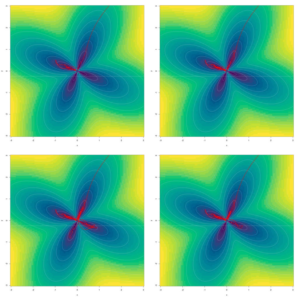
One other playful query that involves thoughts is: Can we observe how the optimization course of “explores” the 4 petals? With some fast experimentation, I arrived at this:

Who says you want chaos to provide a wonderful plot?

A second-order optimizer for neural networks: ADAHESSIAN

On to the one algorithm I’d like to take a look at particularly. Subsequent to somewhat little bit of learning-rate experimentation, I used to be in a position to arrive at a superb outcome after simply thirty-five steps.

test_optim(
    optim = optim_adahessian,
    opt_hparams = list(lr = 0.3),
    test_fn = list(flower, operate() (c(x0 = 20, y0 = 20, xmax = 3, xmin = -3, ymax = 3, ymin = -3))),
    steps = 35
)

Given our current experiences with AdamW although – that means, its “simply not settling in” very near the minimal – we might wish to run an equal take a look at with ADAHESSIAN, as properly. What occurs if we go on optimizing fairly a bit longer – for two-hundred steps, say?

test_optim(
    optim = optim_adahessian,
    opt_hparams = list(lr = 0.3),
    test_fn = list(flower, operate() (c(x0 = 20, y0 = 20, xmax = 3, xmin = -3, ymax = 3, ymin = -3))),
    steps = 200
)

Like AdamW, ADAHESSIAN goes on to “discover” the petals, nevertheless it doesn’t stray as distant from the minimal.

Is that this shocking? I wouldn’t say it’s. The argument is identical as with AdamW, above: Its algorithm has been tuned to carry out properly on giant neural networks, to not resolve a traditional, hand-crafted minimization process.

Now we’ve heard that argument twice already, it’s time to confirm the specific assumption: {that a} traditional second-order algorithm handles this higher. In different phrases, it’s time to revisit L-BFGS.

Better of the classics: Revisiting L-BFGS

To make use of test_optim() with L-BFGS, we have to take somewhat detour. In case you’ve learn the submit on L-BFGS, you could do not forget that with this optimizer, it’s essential to wrap each the decision to the take a look at operate and the analysis of the gradient in a closure. (The reason is that each need to be callable a number of instances per iteration.)

Now, seeing how L-BFGS is a really particular case, and few individuals are doubtless to make use of test_optim() with it sooner or later, it wouldn’t appear worthwhile to make that operate deal with totally different circumstances. For this on-off take a look at, I merely copied and modified the code as required. The outcome, test_optim_lbfgs(), is discovered within the appendix.

In deciding what variety of steps to attempt, we consider that L-BFGS has a special idea of iterations than different optimizers; that means, it could refine its search a number of instances per step. Certainly, from the earlier submit I occur to know that three iterations are ample:

test_optim_lbfgs(
    optim = optim_lbfgs,
    opt_hparams = list(line_search_fn = "strong_wolfe"),
    test_fn = list(flower, operate() (c(x0 = 20, y0 = 20, xmax = 3, xmin = -3, ymax = 3, ymin = -3))),
    steps = 3
)

At this level, after all, I would like to stay with my rule of testing what occurs with “too many steps.” (Although this time, I’ve sturdy causes to imagine that nothing will occur.)

test_optim_lbfgs(
    optim = optim_lbfgs,
    opt_hparams = list(line_search_fn = "strong_wolfe"),
    test_fn = list(flower, operate() (c(x0 = 20, y0 = 20, xmax = 3, xmin = -3, ymax = 3, ymin = -3))),
    steps = 10
)

Speculation confirmed.

And right here ends my playful and subjective introduction to torchopt. I actually hope you appreciated it; however in any case, I feel it’s best to have gotten the impression that here’s a helpful, extensible and likely-to-grow bundle, to be watched out for sooner or later. As all the time, thanks for studying!

Appendix

test_optim_lbfgs <- operate(optim, ...,
                       opt_hparams = NULL,
                       test_fn = "beale",
                       steps = 200,
                       pt_start_color = "#5050FF7F",
                       pt_end_color = "#FF5050FF",
                       ln_color = "#FF0000FF",
                       ln_weight = 2,
                       bg_xy_breaks = 100,
                       bg_z_breaks = 32,
                       bg_palette = "viridis",
                       ct_levels = 10,
                       ct_labels = FALSE,
                       ct_color = "#FFFFFF7F",
                       plot_each_step = FALSE) {


    if (is.character(test_fn)) {
        # get beginning factors
        domain_fn <- get(paste0("domain_",test_fn),
                         envir = asNamespace("torchopt"),
                         inherits = FALSE)
        # get gradient operate
        test_fn <- get(test_fn,
                       envir = asNamespace("torchopt"),
                       inherits = FALSE)
    } else if (is.list(test_fn)) {
        domain_fn <- test_fn[[2]]
        test_fn <- test_fn[[1]]
    }

    # start line
    dom <- domain_fn()
    x0 <- dom[["x0"]]
    y0 <- dom[["y0"]]
    # create tensor
    x <- torch::torch_tensor(x0, requires_grad = TRUE)
    y <- torch::torch_tensor(y0, requires_grad = TRUE)

    # instantiate optimizer
    optim <- do.call(optim, c(list(params = list(x, y)), opt_hparams))

    # with L-BFGS, it's essential to wrap each operate name and gradient analysis in a closure,
    # for them to be callable a number of instances per iteration.
    calc_loss <- operate() {
      optim$zero_grad()
      z <- test_fn(x, y)
      z$backward()
      z
    }

    # run optimizer
    x_steps <- numeric(steps)
    y_steps <- numeric(steps)
    for (i in seq_len(steps)) {
        x_steps[i] <- as.numeric(x)
        y_steps[i] <- as.numeric(y)
        optim$step(calc_loss)
    }

    # put together plot
    # get xy limits

    xmax <- dom[["xmax"]]
    xmin <- dom[["xmin"]]
    ymax <- dom[["ymax"]]
    ymin <- dom[["ymin"]]

    # put together knowledge for gradient plot
    x <- seq(xmin, xmax, size.out = bg_xy_breaks)
    y <- seq(xmin, xmax, size.out = bg_xy_breaks)
    z <- outer(X = x, Y = y, FUN = operate(x, y) as.numeric(test_fn(x, y)))

    plot_from_step <- steps
    if (plot_each_step) {
        plot_from_step <- 1
    }

    for (step in seq(plot_from_step, steps, 1)) {

        # plot background
        image(
            x = x,
            y = y,
            z = z,
            col = hcl.colors(
                n = bg_z_breaks,
                palette = bg_palette
            ),
            ...
        )

        # plot contour
        if (ct_levels > 0) {
            contour(
                x = x,
                y = y,
                z = z,
                nlevels = ct_levels,
                drawlabels = ct_labels,
                col = ct_color,
                add = TRUE
            )
        }

        # plot start line
        points(
            x_steps[1],
            y_steps[1],
            pch = 21,
            bg = pt_start_color
        )

        # plot path line
        lines(
            x_steps[seq_len(step)],
            y_steps[seq_len(step)],
            lwd = ln_weight,
            col = ln_color
        )

        # plot finish level
        points(
            x_steps[step],
            y_steps[step],
            pch = 21,
            bg = pt_end_color
        )
    }
}