Scale back inference time for BERT fashions utilizing neural structure search and SageMaker Automated Mannequin Tuning

On this publish, we display find out how to use neural structure search (NAS) primarily based structural pruning to compress a fine-tuned BERT mannequin to enhance mannequin efficiency and cut back inference occasions. Pre-trained language fashions (PLMs) are present process fast industrial and enterprise adoption within the areas of productiveness instruments, customer support, search and suggestions, enterprise course of automation, and content material creation. Deploying PLM inference endpoints is usually related to greater latency and better infrastructure prices as a result of compute necessities and diminished computational effectivity as a result of giant variety of parameters. Pruning a PLM reduces the scale and complexity of the mannequin whereas retaining its predictive capabilities. Pruned PLMs obtain a smaller reminiscence footprint and decrease latency. We display that by pruning a PLM and buying and selling off parameter rely and validation error for a selected goal process, and are in a position to obtain quicker response occasions when in comparison with the bottom PLM mannequin.

Multi-objective optimization is an space of decision-making that optimizes multiple goal operate, equivalent to reminiscence consumption, coaching time, and compute sources, to be optimized concurrently. Structural pruning is a method to scale back the scale and computational necessities of PLM by pruning layers or neurons/nodes whereas trying to protect mannequin accuracy. By eradicating layers, structural pruning achieves greater compression charges, which ends up in hardware-friendly structured sparsity that reduces runtimes and response occasions. Making use of a structural pruning approach to a PLM mannequin leads to a lighter-weight mannequin with a decrease reminiscence footprint that, when hosted as an inference endpoint in SageMaker, affords improved useful resource effectivity and diminished price when in comparison with the unique fine-tuned PLM.

The ideas illustrated on this publish might be utilized to purposes that use PLM options, equivalent to advice techniques, sentiment evaluation, and engines like google. Particularly, you should utilize this method you probably have devoted machine studying (ML) and information science groups who fine-tune their very own PLM fashions utilizing domain-specific datasets and deploy a lot of inference endpoints utilizing Amazon SageMaker. One instance is an internet retailer who deploys a lot of inference endpoints for textual content summarization, product catalog classification, and product suggestions sentiment classification. One other instance could be a healthcare supplier who makes use of PLM inference endpoints for scientific doc classification, named entity recognition from medical experiences, medical chatbots, and affected person threat stratification.

Answer overview

On this part, we current the general workflow and clarify the method. First, we use an Amazon SageMaker Studio notebook to fine-tune a pre-trained BERT mannequin on a goal process utilizing a domain-specific dataset. BERT (Bidirectional Encoder Representations from Transformers) is a pre-trained language mannequin primarily based on the transformer architecture used for pure language processing (NLP) duties. Neural structure search (NAS) is an method for automating the design of synthetic neural networks and is intently associated to hyperparameter optimization, a broadly used method within the subject of machine studying. The objective of NAS is to seek out the optimum structure for a given drawback by looking over a big set of candidate architectures utilizing strategies equivalent to gradient-free optimization or by optimizing the specified metrics. The efficiency of the structure is usually measured utilizing metrics equivalent to validation loss. SageMaker Automatic Model Tuning (AMT) automates the tedious and sophisticated strategy of discovering the optimum combos of hyperparameters of the ML mannequin that yield the perfect mannequin efficiency. AMT makes use of clever search algorithms and iterative evaluations utilizing a spread of hyperparameters that you just specify. It chooses the hyperparameter values that creates a mannequin that performs the perfect, as measured by efficiency metrics equivalent to accuracy and F-1 rating.

The fine-tuning method described on this publish is generic and might be utilized to any text-based dataset. The duty assigned to the BERT PLM is usually a text-based process equivalent to sentiment evaluation, textual content classification, or Q&A. On this demo, the goal process is a binary classification drawback the place BERT is used to establish, from a dataset that consists of a group of pairs of textual content fragments, whether or not the which means of 1 textual content fragment might be inferred from the opposite fragment. We use the Recognizing Textual Entailment dataset from the GLUE benchmarking suite. We carry out a multi-objective search utilizing SageMaker AMT to establish the sub-networks that supply optimum trade-offs between parameter rely and prediction accuracy for the goal process. When performing a multi-objective search, we begin with defining the accuracy and parameter rely because the targets that we’re aiming to optimize.

Throughout the BERT PLM community, there might be modular, self-contained sub-networks that permit the mannequin to have specialised capabilities equivalent to language understanding and information illustration. BERT PLM makes use of a multi-headed self-attention sub-network and a feed-forward sub-network. A multi-headed, self-attention layer permits BERT to narrate completely different positions of a single sequence with a view to compute a illustration of the sequence by permitting a number of heads to take care of a number of context alerts. The enter is break up into a number of subspaces and self-attention is utilized to every of the subspaces individually. A number of heads in a transformer PLM permit the mannequin to collectively attend to info from completely different illustration subspaces. A feed-forward sub-network is an easy neural community that takes the output from the multi-headed self-attention sub-network, processes the info, and returns the ultimate encoder representations.

The objective of random sub-network sampling is to coach smaller BERT fashions that may carry out nicely sufficient on course duties. We pattern 100 random sub-networks from the fine-tuned base BERT mannequin and consider 10 networks concurrently. The skilled sub-networks are evaluated for the target metrics and the ultimate mannequin is chosen primarily based on the trade-offs discovered between the target metrics. We visualize the Pareto front for the sampled sub-networks, which incorporates the pruned mannequin that provides the optimum trade-off between mannequin accuracy and mannequin measurement. We choose the candidate sub-network (NAS-pruned BERT mannequin) primarily based on the mannequin measurement and mannequin accuracy that we’re keen to commerce off. Subsequent, we host the endpoints, the pre-trained BERT base mannequin, and the NAS-pruned BERT mannequin utilizing SageMaker. To carry out load testing, we use Locust, an open supply load testing software that you would be able to implement utilizing Python. We run load testing on each endpoints utilizing Locust and visualize the outcomes utilizing the Pareto entrance as an example the trade-off between response occasions and accuracy for each fashions. The next diagram offers an summary of the workflow defined on this publish.

Stipulations

For this publish, the next stipulations are required:

You additionally want to extend the service quota to entry a minimum of three cases of ml.g4dn.xlarge cases in SageMaker. The occasion sort ml.g4dn.xlarge is the price environment friendly GPU occasion that permits you to run PyTorch natively. To extend the service quota, full the next steps:

1. On the console, navigate to Service Quotas.
2. For Handle quotas, select Amazon SageMaker, then select View quotas.

3. Seek for “ml-g4dn.xlarge for coaching job utilization” and choose the quota merchandise.
4. Select Request improve at account-level.

5. For Enhance quota worth, enter a worth of 5 or greater.
6. Select Request.

The requested quota approval might take a while to finish relying on the account permissions.

7. Open SageMaker Studio from the SageMaker console.

8. Select System terminal underneath Utilities and recordsdata.

9. Run the next command to clone the GitHub repo to the SageMaker Studio occasion:

   git clone https://github.com/aws/amazon-sagemaker-examples.git

10. Navigate to amazon-sagemaker-examples/hyperparameter_tuning/neural_architecture_search_llm.
11. Open the file nas_for_llm_with_amt.ipynb.
12. Arrange the setting with an ml.g4dn.xlarge occasion and select Choose.

Arrange the pre-trained BERT mannequin

On this part, we import the Recognizing Textual Entailment dataset from the dataset library and break up the dataset into coaching and validation units. This dataset consists of pairs of sentences. The duty of the BERT PLM is to acknowledge, given two textual content fragments, whether or not the which means of 1 textual content fragment might be inferred from the opposite fragment. Within the following instance, we will infer the which means of the primary phrase from the second phrase:

Phrase 1: A person with a beard, carrying a pink shirt with grey sleeves and work gloves, pulling on a rope.
Phrase 2: A bearded man pulls a rope

We load the textual recognizing entailment dataset from the GLUE benchmarking suite by way of the dataset library from Hugging Face inside our coaching script (./coaching.py). We break up the unique coaching dataset from GLUE right into a coaching and validation set. In our method, we fine-tune the bottom BERT mannequin utilizing the coaching dataset, then we carry out a multi-objective search to establish the set of sub-networks that optimally stability between the target metrics. We use the coaching dataset completely for fine-tuning the BERT mannequin. Nevertheless, we use validation information for the multi-objective search by measuring accuracy on the holdout validation dataset.

Fantastic-tune the BERT PLM utilizing a domain-specific dataset

The standard use circumstances for a uncooked BERT mannequin embrace subsequent sentence prediction or masked language modeling. To make use of the bottom BERT mannequin for downstream duties equivalent to textual recognizing entailment, now we have to additional fine-tune the mannequin utilizing a domain-specific dataset. You need to use a fine-tuned BERT mannequin for duties equivalent to sequence classification, query answering, and token classification. Nevertheless, for the needs of this demo, we use the fine-tuned mannequin for binary classification. We fine-tune the pre-trained BERT mannequin with the coaching dataset that we ready beforehand, utilizing the next hyperparameters:

hyperparameters["per_device_train_batch_size"] = 8
hyperparameters["per_device_eval_batch_size"] = 8
hyperparameters["learning_rate"] = 2e-05
hyperparameters["num_train_epochs"] = 5
hyperparameters["save_strategy"] = "epoch"
hyperparameters[
"is_regression"
] = False  # set this to True in case your dataset is a regression dataset, for instance STSB

We save the checkpoint of the mannequin coaching to an Amazon Simple Storage Service (Amazon S3) bucket, in order that the mannequin might be loaded throughout the NAS-based multi-objective search. Earlier than we practice the mannequin, we outline the metrics equivalent to epoch, coaching loss, variety of parameters, and validation error:

session = Session()
s3_bucket = session.default_bucket()
s3_bucket_prefix = "nas_amt/model_checkpoint"
s3_path = f"s3://{s3_bucket}/{s3_bucket_prefix}"

metric_definitions = [
    {"Name": "epoch", "Regex": "epoch: ([0-9.]+)"},
    {"Identify": "training-loss", "Regex": "coaching loss: ([0-9.]+)"},
    {"Identify": "num-parameters", "Regex": "variety of parameters: ([0-9.]+)"},
    {"Identify": "validation-error", "Regex": "validation error: ([0-9.]+)"},
]

sm_args = dict(
    entry_point="coaching.py",
    source_dir=os.path.abspath(""),
    instance_type="ml.g4dn.xlarge",
    instance_count=1,
    py_version="py39",
    framework_version="1.13",
    transformers_version="4.26",
    max_run=3600 * 72,
    position=get_execution_role(),
    checkpoint_local_path="/decide/ml/checkpoints",
    hyperparameters=hyperparameters,
    checkpoint_s3_uri=s3_path,
    metric_definitions=metric_definitions,
)
est = PyTorch(**sm_args)
est.match()

After the fine-tuning course of begins, the coaching job takes round quarter-hour to finish.

Carry out a multi-objective search to pick out sub-networks and visualize the outcomes

Within the subsequent step, we carry out a multi-objective search on the fine-tuned base BERT mannequin by sampling random sub-networks utilizing SageMaker AMT. To entry a sub-network throughout the super-network (the fine-tuned BERT mannequin), we masks out all of the elements of the PLM that aren’t a part of the sub-network. Masking a super-network to seek out sub-networks in a PLM is a method used to isolate and establish patterns of the mannequin’s habits. Be aware that Hugging Face transformers wants the hidden measurement to be a a number of of the variety of heads. The hidden measurement in a transformer PLM controls the scale of the hidden state vector house, which impacts the mannequin’s means to study advanced representations and patterns within the information. In a BERT PLM, the hidden state vector is of a hard and fast measurement (768). We are able to’t change the hidden measurement, and due to this fact the variety of heads must be in [1, 3, 6, 12].

In distinction to single-objective optimization, within the multi-objective setting, we usually don’t have a single answer that concurrently optimizes all targets. As an alternative, we intention to gather a set of options that dominate all different options in a minimum of one goal (equivalent to validation error). Now we will begin the multi-objective search via AMT by setting the metrics that we wish to cut back (validation error and variety of parameters). The random sub-networks are outlined by the parameter max_jobs and the variety of simultaneous jobs is outlined by the parameter max_parallel_jobs. The code to load the mannequin checkpoint and consider the sub-network is offered within the evaluate_subnetwork.py script.

# Most variety of sub-networks we are going to consider
max_jobs = 100
max_parallel_jobs = 5

# Entry level script to load the super-network and consider a sub-network
entry_point = "evaluate_subnetwork.py"

# Command line arguments for the entry level script
hyperparameters = {"model_name_or_path": model_type, "output_dir": "./tmp", "task_name": "rte"}

# Outline the metric we wish to decrease
metric_definitions = [
    {"Name": "num-parameters", "Regex": "number of parameters: ([0-9.]+)"},
    {"Identify": "validation-error", "Regex": "validation error: ([0-9.]+)"},
]

# Outline HuggingFace estimator
estimator = HuggingFace(
    entry_point=entry_point,
    source_dir="./",
    instance_type="ml.g4dn.xlarge",  # occasion sorts for the SageMaker coaching jobs
    instance_count=1,
    py_version="py39",
    framework_version="1.13",
    pytorch_version="1.13",
    transformers_version="4.26",
    max_run=3600 * 72,
    position=get_execution_role(),
    volume_size=125,
    model_uri=s3_path,
    hyperparameters=hyperparameters,
)

current_time = datetime.now().strftime("%m-%d-%Y-%H-%M-%S")
tuning_job_name = f"nas-search-{current_time}"

# Search house to outline sub-networks
hyperparameter_ranges = {
    "num_layers": IntegerParameter(0, 12),
    # To satisfy HuggingFace constraints, we will solely set the variety of head to those values
    "num_heads": CategoricalParameter([1, 3, 6, 12]),
    "num_units": IntegerParameter(0, 3072),
}

# Outline AMT Tuner object
my_tuner = HyperparameterTuner(
    estimator=estimator,
    objective_metric_name="validation-error",
    hyperparameter_ranges=hyperparameter_ranges,
    metric_definitions=metric_definitions,
    max_jobs=max_jobs,
    technique="Random",
    random_seed=seed,
    objective_type="Decrease",
    max_parallel_jobs=max_parallel_jobs,
)

# Begin hyperparameter tuning job
my_tuner.match(job_name=tuning_job_name)

The AMT tuning job takes roughly 2 hours and 20 minutes to run. After the AMT tuning job runs efficiently, we parse the job’s historical past and accumulate the sub-network’s configurations, equivalent to variety of heads, variety of layers, variety of items, and the corresponding metrics equivalent to validation error and variety of parameters. The next screenshot reveals the abstract of a profitable AMT tuner job.

Subsequent, we visualize the outcomes utilizing a Pareto set (also referred to as Pareto frontier or Pareto optimum set), which helps us establish optimum units of sub-networks that dominate all different sub-networks within the goal metric (validation error):

historical past = my_tuner.analytics().dataframe()
information = []
configs = []
for i, t in enumerate(my_tuner.analytics().training_job_summaries()):
    jn = t["TrainingJobName"]
    df = sagemaker.analytics.TrainingJobAnalytics(jn).dataframe()

    row = historical past[history["TrainingJobName"] == jn]
    config = {
        "num-heads": int(row["num_heads"].iloc[0].strip('"')),
        "num-layers": int(row["num_layers"]),
        "num-units": int(row["num_units"]),
    }
    configs.append(config)

    p = []
    for j, metric in enumerate(metric_definitions):
        metric_name = metric["Name"]
        if "metric_name" not in df.keys():
            proceed
        y = float(df[df["metric_name"] == metric_name]["value"])
        p.append(y)
    if len(p) > 0:
        information.append(p)

information = np.array(information)

First, we accumulate the info from the AMT tuning job. Then then we plot the Pareto set utilizing matplotlob.pyplot with variety of parameters within the x axis and validation error within the y axis. This means that after we transfer from one sub-network of the Pareto set to a different, we should both sacrifice efficiency or mannequin measurement however enhance the opposite. Finally, the Pareto set offers us the flexibleness to decide on the sub-network that most accurately fits our preferences. We are able to determine how a lot we wish to cut back the scale of our community and the way a lot efficiency we’re keen to sacrifice.

import matplotlib.pyplot as plt
from multi_objective import get_pareto_optimal

# get outcomes of the un-pruned community
df = sagemaker.analytics.TrainingJobAnalytics(est.jobs[0].identify).dataframe()
validation_error_unpruned_network = float(df[df["metric_name"] == "validation-error"].worth.min())
params_unpruned_network = int(df[df["metric_name"] == "num-parameters"].worth.min())
plt.scatter(
params_unpruned_network,
validation_error_unpruned_network,
marker="o",
s=80,
facecolors="none",
edgecolors="C3",
linewidth=2,
label="un-pruned super-network",
)
# get Pareto optimum factors
idx = get_pareto_optimal(information)
x = information[idx, 0]
y = information[idx, 1]
plt.scatter(
x,
y,
marker="o",
s=80,
facecolors="none",
edgecolors="C0",
linewidth=2,
label="Pareto entrance (sub-networks)",
)
plt.xlabel("variety of parameters")
plt.ylabel("validation error")
plt.legend()
plt.xscale("log")
plt.grid(linewidth="1", alpha=0.4, which="each")

Deploy the fine-tuned BERT mannequin and the NAS-optimized sub-network mannequin utilizing SageMaker

Subsequent, we deploy the biggest mannequin in our Pareto set that results in the smallest quantity of efficiency degeneration to a SageMaker endpoint. The very best mannequin is the one that gives an optimum trade-off between the validation error and the variety of parameters for our use case.

# Let's take the biggest mannequin within the Pareto set
indicies = np.arange(len(configs))[idx]
pareto_optimal_sub_networks = [configs[i] for i in indicies]
config_to_deploy = pareto_optimal_sub_networks[-1]  

from sagemaker.huggingface.mannequin import HuggingFaceModel

# create Hugging Face Mannequin Class
huggingface_model = HuggingFaceModel(
    model_data=s3_path + "/mannequin.tar.gz",
    position=get_execution_role(),
    transformers_version="4.26",
    pytorch_version="1.13",
    py_version="py39",
    entry_point="inference.py",
    source_dir="./",
    env={"SM_HPS": json.dumps(config_to_deploy)},
)

# deploy mannequin to SageMaker Inference
predictor = huggingface_model.deploy(initial_instance_count=1, instance_type="ml.g4dn.xlarge")

Mannequin comparability

We took a pre-trained base BERT mannequin, fine-tuned it utilizing a domain-specific dataset, ran a NAS search to establish dominant sub-networks primarily based on the target metrics, and deployed the pruned mannequin on a SageMaker endpoint. As well as, we took the pre-trained base BERT mannequin and deployed the bottom mannequin on a second SageMaker endpoint. Subsequent, we ran load-testing utilizing Locust on each inference endpoints and evaluated the efficiency when it comes to response time.

First, we import the mandatory Locust and Boto3 libraries. Then we assemble a request metadata and report the beginning time for use for load testing. Then the payload is handed to the SageMaker endpoint invoke API by way of the BotoClient to simulate actual consumer requests. We use Locust to spawn a number of digital customers to ship requests in parallel and measure the endpoint efficiency underneath the load. Checks are run by rising the variety of customers for every of the 2 endpoints, respectively. After the exams are accomplished, Locust outputs a request statistics CSV file for every of the deployed fashions.

def ship(self):
        request_meta = {
            "request_type": "InvokeEndpoint",
            "identify": "SageMaker",
            "start_time": time.time(),
            "response_length": 0,
            "response": None,
            "context": {},
            "exception": None,
        }
        start_perf_counter = time.perf_counter()

        attempt:
            response = self.sagemaker_client.invoke_endpoint(
                EndpointName=self.endpoint_name,
                Physique=self.payload,
                ContentType=self.content_type,
            )
            logging.information(response["Body"].learn())
        besides Exception as e:
            request_meta["exception"] = e

        request_meta["response_time"] = (
            time.perf_counter() - start_perf_counter
        ) * 1000

        occasions.request.hearth(**request_meta)

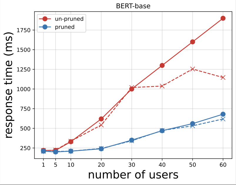
Subsequent, we generate the response time plots from the CSV recordsdata downloaded after working the exams with Locust. The aim of plotting the response time vs. the variety of customers is to investigate the load testing outcomes by visualizing the affect of the response time of the mannequin endpoints. Within the following chart, we will see that the NAS-pruned mannequin endpoint achieves a decrease response time in comparison with the bottom BERT mannequin endpoint.

Within the second chart, which is an extension of the primary chart, we observe that after round 70 customers, SageMaker begins to throttle the bottom BERT mannequin endpoint and throws an exception. Nevertheless, for the NAS-pruned mannequin endpoint, the throttling occurs between 90–100 customers and with a decrease response time.

From the 2 charts, we observe that the pruned mannequin has a quicker response time and scales higher when in comparison with the unpruned mannequin. As we scale the variety of inference endpoints, as is the case with customers who deploy a lot of inference endpoints for his or her PLM purposes, the price advantages and efficiency enchancment begin to turn out to be fairly substantial.

Clear up

To delete the SageMaker endpoints for the fine-tuned base BERT mannequin and the NAS-pruned mannequin, full the next steps:

1. On the SageMaker console, select Inference and Endpoints within the navigation pane.
2. Choose the endpoint and delete it.

Alternatively, from the SageMaker Studio pocket book, run the next instructions by offering the endpoint names:

predictor.delete_model()
predictor.delete_endpoint()

Conclusion

On this publish, we mentioned find out how to use NAS to prune a fine-tuned BERT mannequin. We first skilled a base BERT mannequin utilizing domain-specific information and deployed it to a SageMaker endpoint. We carried out a multi-objective search on the fine-tuned base BERT mannequin utilizing SageMaker AMT for a goal process. We visualized the Pareto entrance and chosen the Pareto optimum NAS-pruned BERT mannequin and deployed the mannequin to a second SageMaker endpoint. We carried out load testing utilizing Locust to simulate customers querying each the endpoints, and measured and recorded the response occasions in a CSV file. We plotted the response time vs. the variety of customers for each the fashions.

We noticed that the pruned BERT mannequin carried out considerably higher in each response time and occasion throttling threshold. We concluded that the NAS-pruned mannequin was extra resilient to an elevated load on the endpoint, sustaining a decrease response time whilst extra customers confused the system in comparison with the bottom BERT mannequin. You may apply the NAS approach described on this publish to any giant language mannequin to discover a pruned mannequin that may carry out the goal process with considerably decrease response time. You may additional optimize the method through the use of latency as a parameter along with validation loss.

Though we use NAS on this publish, quantization is one other widespread method used to optimize and compress PLM fashions. Quantization reduces the precision of the weights and activations in a skilled community from 32-bit floating level to decrease bit widths equivalent to 8-bit or 16-bit integers, which ends up in a compressed mannequin that generates quicker inference. Quantization doesn’t cut back the variety of parameters; as an alternative it reduces the precision of the present parameters to get a compressed mannequin. NAS pruning removes redundant networks in a PLM, which creates a sparse mannequin with fewer parameters. Sometimes, NAS pruning and quantization are used collectively to compress giant PLMs to take care of mannequin accuracy, cut back validation losses whereas bettering efficiency, and cut back mannequin measurement. The opposite generally used strategies to scale back the scale of PLMs embrace knowledge distillation, matrix factorization, and distillation cascades.

The method proposed within the blogpost is appropriate for groups that use SageMaker to coach and fine-tune the fashions utilizing domain-specific information and deploy the endpoints to generate inference. If you happen to’re in search of a completely managed service that provides a selection of high-performing basis fashions wanted to construct generative AI purposes, think about using Amazon Bedrock. If you happen to’re in search of pre-trained, open supply fashions for a variety of enterprise use circumstances and wish to entry answer templates and instance notebooks, think about using Amazon SageMaker JumpStart. A pre-trained model of the Hugging Face BERT base cased mannequin that we used on this publish can also be obtainable from SageMaker JumpStart.

In regards to the Authors

Aparajithan Vaidyanathan is a Principal Enterprise Options Architect at AWS. He’s a Cloud Architect with 24+ years of expertise designing and growing enterprise, large-scale and distributed software program techniques. He makes a speciality of Generative AI and Machine Studying Information Engineering. He’s an aspiring marathon runner and his hobbies embrace mountain climbing, bike using and spending time along with his spouse and two boys.

Aaron Klein is a Sr Utilized Scientist at AWS engaged on automated machine studying strategies for deep neural networks.

Jacek Golebiowski is a Sr Utilized Scientist at AWS.