Implementing Delicate Nearest Neighbor Loss in PyTorch | by Abien Fred Agarap | Nov, 2023

The category neighborhood of a dataset will be discovered utilizing smooth nearest neighbor loss

On this article, we talk about how you can implement the smooth nearest neighbor loss which we additionally talked about here.

Representation studying is the duty of studying essentially the most salient options in a given dataset by a deep neural community. It’s normally an implicit process carried out in a supervised studying paradigm, and it’s a essential issue within the success of deep studying (Krizhevsky et al., 2012; He et al., 2016; Simonyan et al., 2014). In different phrases, illustration studying automates the method of characteristic extraction. With this, we are able to use the discovered representations for downstream duties similar to classification, regression, and synthesis.

We will additionally affect how the discovered representations are fashioned to cater particular use circumstances. Within the case of classification, the representations are primed to have information factors from the identical class to flock collectively, whereas for technology (e.g. in GANs), the representations are primed to have factors of actual information flock with the synthesized ones.

In the identical sense, we now have loved the usage of principal parts evaluation (PCA) to encode options for downstream duties. Nevertheless, we wouldn’t have any class or label data in PCA-encoded representations, therefore the efficiency on downstream duties could also be additional improved. We will enhance the encoded representations by approximating the category or label data in it by studying the neighborhood construction of the dataset, i.e. which options are clustered collectively, and such clusters would suggest that the options belong to the identical class as per the clustering assumption within the semi-supervised studying literature (Chapelle et al., 2009).

To combine the neighborhood construction within the representations, manifold studying strategies have been launched similar to regionally linear embeddings or LLE (Roweis & Saul, 2000), neighborhood parts evaluation or NCA (Hinton et al., 2004), and t-stochastic neighbor embedding or t-SNE (Maaten & Hinton, 2008).

Nevertheless, the aforementioned manifold studying strategies have their very own drawbacks. For example, each LLE and NCA encode linear embeddings as an alternative of nonlinear embeddings. In the meantime, t-SNE embeddings end result to completely different buildings relying on the hyperparameters used.

To keep away from such drawbacks, we are able to use an improved NCA algorithm which is the smooth nearest neighbor loss or SNNL (Salakhutdinov & Hinton, 2007; Frosst et al., 2019). The SNNL improves the NCA algorithm by introducing nonlinearity, and it’s computed for every hidden layer of a neural community as an alternative of solely on the final encoding layer. This loss perform is used to optimize the entanglement of factors in a dataset.

On this context, entanglement is outlined as how shut class-similar information factors to one another are in comparison with class-different information factors. A low entanglement implies that class-similar information factors are a lot nearer to one another than class-different information factors (see Determine 1). Having such a set of knowledge factors will render downstream duties a lot simpler to perform with a good higher efficiency. Frosst et al. (2019) expanded the SNNL goal by introducing a temperature issue T. Thus giving us the next as the ultimate loss perform,

the place d is a distance metric on both uncooked enter options or hidden layer representations of a neural community, and T is the temperature issue that’s straight proportional to the distances amongst information factors in a hidden layer. For this implementation, we use the cosine distance as our distance metric for extra secure computations.

The aim of this text is to assist readers perceive and implement the smooth nearest neighbor loss, and so we will dissect the loss perform to be able to perceive it higher.

Distance Metric

The very first thing we should always compute are the distances amongst information factors, which can be both the uncooked enter options or hidden layer representations of the community.

For our implementation, we use the cosine distance metric (Determine 3) for extra secure computations. On the time being, allow us to ignore the denoted subsets ij and ik within the determine above, and allow us to simply concentrate on computing the cosine distance amongst our enter information factors. We accomplish this by the next PyTorch code:

normalized_a = torch.nn.purposeful.normalize(options, dim=1, p=2)
normalized_b = torch.nn.purposeful.normalize(options, dim=1, p=2)
normalized_b = torch.conj(normalized_b).T
product = torch.matmul(normalized_a, normalized_b)
distance_matrix = torch.sub(torch.tensor(1.0), product)

Within the code snippet above, we first normalize the enter options in strains 1 and a pair of utilizing Euclidean norm. Then in line 3, we get the conjugate transpose of the second set of the normalized enter options. We compute the conjugate transpose to account for complex vectors. In strains 4 and 5, we compute the cosine similarity and distance of the enter options.

Concretely, think about the next set of options,

tensor([[ 1.0999, -0.9438,  0.7996, -0.4247],
[ 1.2150, -0.2953,  0.0417, -1.2913],
[ 1.3218,  0.4214, -0.1541,  0.0961],
[-0.7253,  1.1685, -0.1070,  1.3683]])

Utilizing the gap metric we outlined above, we acquire the next distance matrix,

tensor([[ 0.0000e+00,  2.8502e-01,  6.2687e-01,  1.7732e+00],
[ 2.8502e-01,  0.0000e+00,  4.6293e-01,  1.8581e+00],
[ 6.2687e-01,  4.6293e-01, -1.1921e-07,  1.1171e+00],
[ 1.7732e+00,  1.8581e+00,  1.1171e+00, -1.1921e-07]])

Sampling Chance

We will now compute the matrix that represents the chance of choosing every characteristic given its pairwise distances to all different options. That is merely the chance of choosing i factors primarily based on the distances between i and j or okay factors.

We will compute this by the next code:

pairwise_distance_matrix = torch.exp(
-(distance_matrix / temperature)
) - torch.eye(options.form[0]).to(mannequin.gadget)

The code first calculates the exponential of the unfavorable of the gap matrix divided by the temperature issue, scaling the values to constructive values. The temperature issue dictates how you can management the significance given to the distances between pairs of factors, for example, at low temperatures, the loss is dominated by small distances whereas precise distances between broadly separated representations turn into much less related.

Previous to the subtraction of torch.eye(options.form[0]) (aka diagonal matrix), the tensor was as follows,

tensor([[1.0000, 0.7520, 0.5343, 0.1698],
[0.7520, 1.0000, 0.6294, 0.1560],
[0.5343, 0.6294, 1.0000, 0.3272],
[0.1698, 0.1560, 0.3272, 1.0000]])

We subtract a diagonal matrix from the gap matrix to take away all self-similarity phrases (i.e. the gap or similarity of every level to itself).

Subsequent, we are able to compute the sampling chance for every pair of knowledge factors by the next code:

pick_probability = pairwise_distance_matrix / (
torch.sum(pairwise_distance_matrix, 1).view(-1, 1)
+ stability_epsilon
)

Masked Sampling Chance

Up to now, the sampling chance we now have computed doesn’t comprise any label data. We combine the label data into the sampling chance by masking it with the dataset labels.

First, we now have to derive a pairwise matrix out of the label vectors:

masking_matrix = torch.squeeze(
torch.eq(labels, labels.unsqueeze(1)).float()
)

We apply the masking matrix to make use of the label data to isolate the possibilities for factors that belong to the identical class:

masked_pick_probability = pick_probability * masking_matrix

Subsequent, we compute the sum chance for sampling a selected characteristic by computing the sum of the masked sampling chance per row,

summed_masked_pick_probability = torch.sum(masked_pick_probability, dim=1)

Lastly, we are able to compute the logarithm of the sum of the sampling chances for options for computational comfort with an extra computational stability variable, and get the common to behave as the closest neighbor loss for the community,

snnl = torch.imply(
-torch.log(summed_masked_pick_probability + stability_epsilon
)

We will now string these parts collectively in a ahead cross perform to compute the smooth nearest neighbor loss throughout all layers of a deep neural community,

def ahead(
self,
mannequin: torch.nn.Module,
options: torch.Tensor,
labels: torch.Tensor,
outputs: torch.Tensor,
epoch: int,
) -> Tuple:
if self.use_annealing:
self.temperature = 1.0 / ((1.0 + epoch) ** 0.55)
primary_loss = self.primary_criterion(
outputs, options if self.unsupervised else labels
)
activations = self.compute_activations(mannequin=mannequin, options=options)
layers_snnl = []
for key, worth in activations.gadgets():
worth = worth[:, : self.code_units]
distance_matrix = self.pairwise_cosine_distance(options=worth)
pairwise_distance_matrix = self.normalize_distance_matrix(
options=worth, distance_matrix=distance_matrix
)
pick_probability = self.compute_sampling_probability(
pairwise_distance_matrix
)
summed_masked_pick_probability = self.mask_sampling_probability(
labels, pick_probability
)
snnl = torch.imply(
-torch.log(self.stability_epsilon + summed_masked_pick_probability)
)
layers_snnl.append(snnl)
snn_loss = torch.stack(layers_snnl).sum()
train_loss = torch.add(primary_loss, torch.mul(self.issue, snn_loss))
return train_loss, primary_loss, snn_loss

Visualizing Disentangled Representations

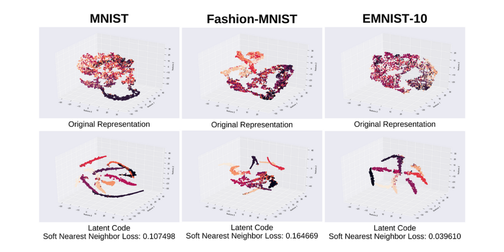
We educated an autoencoder with the smooth nearest neighbor loss, and visualize its discovered disentangled representations. The autoencoder had (x-500–500–2000-d-2000–500–500-x) models, and was educated on a small labelled subset of the MNIST, Style-MNIST, and EMNIST-Balanced datasets. That is to simulate the shortage of labelled examples since autoencoders are alleged to be unsupervised fashions.

We solely visualized an arbitrarily chosen 10 clusters for simpler and cleaner visualization of the EMNIST-Balanced dataset. We will see within the determine above that the latent code illustration grew to become extra clustering-friendly by having a set of well-defined clusters as indicated by cluster dispersion and proper cluster assignments as indicated by cluster colours.

Closing Remarks

On this article, we dissected the smooth nearest neighbor loss perform as to how we might implement it in PyTorch.

The smooth nearest neighbor loss was first launched by Salakhutdinov & Hinton (2007) the place it was used to compute the loss on the latent code (bottleneck) illustration of an autoencoder, after which the stated illustration was used for downstream kNN classification process.

Frosst, Papernot, & Hinton (2019) then expanded the smooth nearest neighbor loss by introducing a temperature issue and by computing the loss throughout all layers of a neural community.

Lastly, we employed an annealing temperature issue for the smooth nearest neighbor loss to additional enhance the discovered disentangled representations of a community, and in addition pace up the disentanglement course of (Agarap & Azcarraga, 2020).

The complete code implementation is obtainable in GitLab.

References

• Agarap, Abien Fred, and Arnulfo P. Azcarraga. “Enhancing k-means clustering efficiency with disentangled inside representations.” 2020 Worldwide Joint Convention on Neural Networks (IJCNN). IEEE, 2020.
• Chapelle, Olivier, Bernhard Scholkopf, and Alexander Zien. “Semi-supervised studying (chapelle, o. et al., eds.; 2006)[book reviews].” IEEE Transactions on Neural Networks 20.3 (2009): 542–542.
• Frosst, Nicholas, Nicolas Papernot, and Geoffrey Hinton. “Analyzing and bettering representations with the smooth nearest neighbor loss.” Worldwide convention on machine studying. PMLR, 2019.
• Goldberger, Jacob, et al. “Neighbourhood parts evaluation.” Advances in neural data processing methods. 2005.
• He, Kaiming, et al. “Deep residual studying for picture recognition.” Proceedings of the IEEE convention on pc imaginative and prescient and sample recognition. 2016.
• Hinton, G., et al. “Neighborhood parts evaluation.” Proc. NIPS. 2004.
• Krizhevsky, Alex, Ilya Sutskever, and Geoffrey E. Hinton. “Imagenet classification with deep convolutional neural networks.” Advances in neural data processing methods 25 (2012).
• Roweis, Sam T., and Lawrence Okay. Saul. “Nonlinear dimensionality discount by regionally linear embedding.” science 290.5500 (2000): 2323–2326.
• Salakhutdinov, Ruslan, and Geoff Hinton. “Studying a nonlinear embedding by preserving class neighbourhood construction.” Synthetic Intelligence and Statistics. 2007.
• Simonyan, Karen, and Andrew Zisserman. “Very deep convolutional networks for large-scale picture recognition.” arXiv preprint arXiv:1409.1556 (2014).
• Van der Maaten, Laurens, and Geoffrey Hinton. “Visualizing information utilizing t-SNE.” Journal of machine studying analysis 9.11 (2008).