Fundamentals Of Statistics For Information Scientists and Analysts

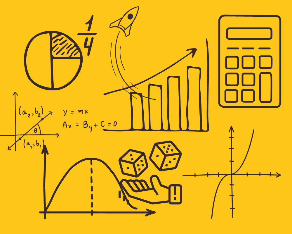
Picture by Editor

As Karl Pearson, a British mathematician has as soon as said, Statistics is the grammar of science and this holds particularly for Laptop and Info Sciences, Bodily Science, and Organic Science. If you find yourself getting began together with your journey in Information Science or Information Analytics, having statistical information will enable you to to higher leverage information insights.

“Statistics is the grammar of science.” Karl Pearson

The significance of statistics in information science and information analytics can’t be underestimated. Statistics gives instruments and strategies to seek out construction and to provide deeper information insights. Each Statistics and Arithmetic love info and hate guesses. Realizing the basics of those two essential topics will help you assume critically, and be inventive when utilizing the information to resolve enterprise issues and make data-driven choices. On this article, I’ll cowl the next Statistics subjects for information science and information analytics:

- Random variables

- Chance distribution features (PDFs)

- Imply, Variance, Commonplace Deviation

- Covariance and Correlation 

- Bayes Theorem

- Linear Regression and Odd Least Squares (OLS)

- Gauss-Markov Theorem

- Parameter properties (Bias, Consistency, Effectivity)

- Confidence intervals

- Speculation testing

- Statistical significance 

- Sort I & Sort II Errors

- Statistical exams (Pupil's t-test, F-test)

- p-value and its limitations

- Inferential Statistics 

- Central Restrict Theorem & Regulation of Giant Numbers

- Dimensionality discount strategies (PCA, FA)

When you have no prior Statistical information and also you need to establish and be taught the important statistical ideas from the scratch, to organize in your job interviews, then this text is for you. This text can even be learn for anybody who needs to refresh his/her statistical information.

Welcome to LunarTech.ai, the place we perceive the facility of job-searching methods within the dynamic subject of Information Science and AI. We dive deep into the techniques and techniques required to navigate the aggressive job search course of. Whether or not it’s defining your profession objectives, customizing utility supplies, or leveraging job boards and networking, our insights present the steerage that you must land your dream job.

Making ready for information science interviews? Worry not! We shine a lightweight on the intricacies of the interview course of, equipping you with the information and preparation mandatory to extend your probabilities of success. From preliminary cellphone screenings to technical assessments, technical interviews, and behavioral interviews, we go away no stone unturned.

At LunarTech.ai, we transcend the idea. We’re your springboard to unparalleled success within the tech and information science realm. Our complete studying journey is tailor-made to suit seamlessly into your life-style, permitting you to strike the proper steadiness between private {and professional} commitments whereas buying cutting-edge expertise. With our dedication to your profession progress, together with job placement help, skilled resume constructing, and interview preparation, you’ll emerge as an industry-ready powerhouse.

Be part of our group of formidable people as we speak and embark on this thrilling information science journey collectively. With LunarTech.ai, the longer term is shiny, and also you maintain the keys to unlock boundless alternatives.

The idea of random variables varieties the cornerstone of many statistical ideas. It is perhaps laborious to digest its formal mathematical definition however merely put, a random variable is a strategy to map the outcomes of random processes, reminiscent of flipping a coin or rolling a cube, to numbers. As an illustration, we are able to outline the random means of flipping a coin by random variable X which takes a price 1 if the result if heads and 0 if the result is tails.

On this instance, we now have a random means of flipping a coin the place this experiment can produce two potential outcomes: {0,1}. This set of all potential outcomes is named the pattern house of the experiment. Every time the random course of is repeated, it’s known as an occasion. On this instance, flipping a coin and getting a tail as an final result is an occasion. The possibility or the probability of this occasion occurring with a selected final result is named the likelihood of that occasion. A likelihood of an occasion is the probability {that a} random variable takes a selected worth of x which might be described by P(x). Within the instance of flipping a coin, the probability of getting heads or tails is identical, that’s 0.5 or 50%. So we now have the next setting:

the place the likelihood of an occasion, on this instance, can solely take values within the vary [0,1].

The significance of statistics in information science and information analytics can’t be underestimated. Statistics gives instruments and strategies to seek out construction and to provide deeper information insights.

To grasp the ideas of imply, variance, and plenty of different statistical subjects, it is very important be taught the ideas of inhabitants and pattern. The inhabitants is the set of all observations (people, objects, occasions, or procedures) and is normally very massive and various, whereas a pattern is a subset of observations from the inhabitants that ideally is a real illustration of the inhabitants.

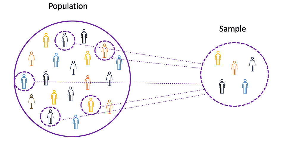
Picture Supply: The Creator

On condition that experimenting with a complete inhabitants is both unattainable or just too costly, researchers or analysts use samples moderately than the complete inhabitants of their experiments or trials. To make it possible for the experimental outcomes are dependable and maintain for the complete inhabitants, the pattern must be a real illustration of the inhabitants. That’s, the pattern must be unbiased. For this goal, one can use statistical sampling strategies reminiscent of Random Sampling, Systematic Sampling, Clustered Sampling, Weighted Sampling, and Stratified Sampling.

Imply

The imply, often known as the typical, is a central worth of a finite set of numbers. Let’s assume a random variable X within the information has the next values:

the place N is the variety of observations or information factors within the pattern set or just the information frequency. Then the pattern imply outlined by ?, which could be very typically used to approximate the inhabitants imply, might be expressed as follows:

The imply can be known as expectation which is commonly outlined by E() or random variable with a bar on the highest. For instance, the expectation of random variables X and Y, that’s E(X) and E(Y), respectively, might be expressed as follows:

import numpy as np
import math
x = np.array([1,3,5,6])
mean_x = np.imply(x)
# in case the information incorporates Nan values
x_nan = np.array([1,3,5,6, math.nan])
mean_x_nan = np.nanmean(x_nan)

Variance

The variance measures how far the information factors are unfold out from the typical worth, and is the same as the sum of squares of variations between the information values and the typical (the imply). Moreover, the inhabitants variance, might be expressed as follows:

x = np.array([1,3,5,6])
variance_x = np.var(x)

# right here that you must specify the levels of freedom (df) max variety of logically unbiased information factors which have freedom to fluctuate
x_nan = np.array([1,3,5,6, math.nan])
mean_x_nan = np.nanvar(x_nan, ddof = 1)

For deriving expectations and variances of various fashionable likelihood distribution features, check out this Github repo.

Commonplace Deviation

The usual deviation is just the sq. root of the variance and measures the extent to which information varies from its imply. The usual deviation outlined by sigma might be expressed as follows:

Commonplace deviation is commonly most popular over the variance as a result of it has the identical unit as the information factors, which suggests you possibly can interpret it extra simply.

x = np.array([1,3,5,6])
variance_x = np.std(x)

x_nan = np.array([1,3,5,6, math.nan])
mean_x_nan = np.nanstd(x_nan, ddof = 1)

Covariance

The covariance is a measure of the joint variability of two random variables and describes the connection between these two variables. It’s outlined because the anticipated worth of the product of the 2 random variables’ deviations from their means. The covariance between two random variables X and Z might be described by the next expression, the place E(X) and E(Z) characterize the technique of X and Z, respectively.

Covariance can take detrimental or optimistic values in addition to worth 0. A optimistic worth of covariance signifies that two random variables are inclined to fluctuate in the identical path, whereas a detrimental worth means that these variables fluctuate in reverse instructions. Lastly, the worth 0 signifies that they don’t fluctuate collectively.

x = np.array([1,3,5,6])
y = np.array([-2,-4,-5,-6])
#this may return the covariance matrix of x,y containing x_variance, y_variance on diagonal parts and covariance of x,y
cov_xy = np.cov(x,y)

Correlation

The correlation can be a measure for relationship and it measures each the power and the path of the linear relationship between two variables. If a correlation is detected then it means that there’s a relationship or a sample between the values of two goal variables. Correlation between two random variables X and Z are equal to the covariance between these two variables divided to the product of the usual deviations of those variables which might be described by the next expression.

Correlation coefficients’ values vary between -1 and 1. Understand that the correlation of a variable with itself is at all times 1, that’s Cor(X, X) = 1. One other factor to bear in mind when decoding correlation is to not confuse it with causation, given {that a} correlation is just not causation. Even when there’s a correlation between two variables, you can not conclude that one variable causes a change within the different. This relationship could possibly be coincidental, or a 3rd issue is perhaps inflicting each variables to vary.

x = np.array([1,3,5,6])
y = np.array([-2,-4,-5,-6])
corr = np.corrcoef(x,y)

A operate that describes all of the potential values, the pattern house, and the corresponding possibilities {that a} random variable can take inside a given vary, bounded between the minimal and most potential values, is named a likelihood distribution operate (pdf) or likelihood density. Each pdf must fulfill the next two standards:

the place the primary criterium states that each one possibilities needs to be numbers within the vary of [0,1] and the second criterium states that the sum of all potential possibilities needs to be equal to 1.

Chance features are normally labeled into two classes: discrete and steady. Discrete distribution operate describes the random course of with countable pattern house, like within the case of an instance of tossing a coin that has solely two potential outcomes. Steady distribution operate describes the random course of with steady pattern house. Examples of discrete distribution features are Bernoulli, Binomial, Poisson, Discrete Uniform. Examples of steady distribution features are Normal, Continuous Uniform, Cauchy.

Binomial Distribution

The binomial distribution is the discrete likelihood distribution of the variety of successes in a sequence of n unbiased experiments, every with the boolean-valued final result: success (with likelihood p) or failure (with likelihood q = 1 ? p). Let’s assume a random variable X follows a Binomial distribution, then the likelihood of observing okay successes in n unbiased trials might be expressed by the next likelihood density operate:

The binomial distribution is beneficial when analyzing the outcomes of repeated unbiased experiments, particularly if one is within the likelihood of assembly a selected threshold given a selected error fee.

Binomial Distribution Imply & Variance

The determine beneath visualizes an instance of Binomial distribution the place the variety of unbiased trials is the same as 8 and the likelihood of success in every trial is the same as 16%.

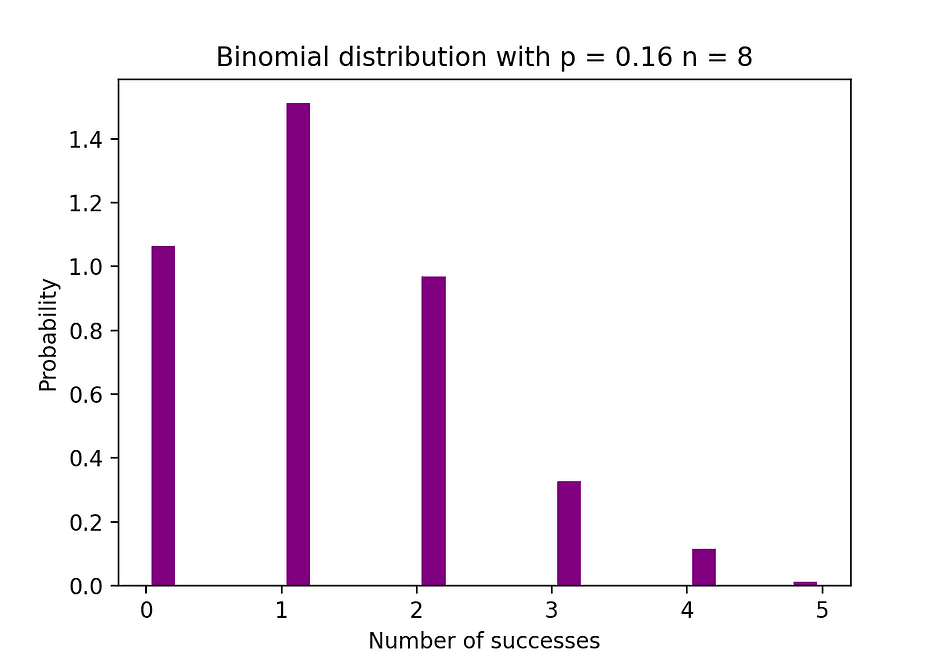
Picture Supply: The Creator

# Random Era of 1000 unbiased Binomial samples
import numpy as np
n = 8
p = 0.16
N = 1000
X = np.random.binomial(n,p,N)
# Histogram of Binomial distribution
import matplotlib.pyplot as plt
counts, bins, ignored = plt.hist(X, 20, density = True, rwidth = 0.7, colour="purple")
plt.title("Binomial distribution with p = 0.16 n = 8")
plt.xlabel("Variety of successes")
plt.ylabel("Chance")
plt.present()

Poisson Distribution

The Poisson distribution is the discrete likelihood distribution of the variety of occasions occurring in a specified time interval, given the typical variety of occasions the occasion happens over that point interval. Let’s assume a random variable X follows a Poisson distribution, then the likelihood of observing okay occasions over a time interval might be expressed by the next likelihood operate:

the place e is Euler’s number and ? lambda, the arrival fee parameter is the anticipated worth of X. Poisson distribution operate could be very fashionable for its utilization in modeling countable occasions occurring inside a given time interval.

Poisson Distribution Imply & Variance

For instance, Poisson distribution can be utilized to mannequin the variety of clients arriving within the store between 7 and 10 pm, or the variety of sufferers arriving in an emergency room between 11 and 12 pm. The determine beneath visualizes an instance of Poisson distribution the place we rely the variety of Internet guests arriving on the web site the place the arrival fee, lambda, is assumed to be equal to 7 minutes.

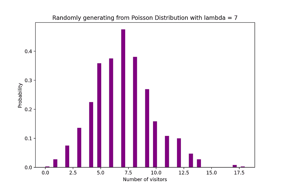
Picture Supply: The Creator

# Random Era of 1000 unbiased Poisson samples
import numpy as np
lambda_ = 7
N = 1000
X = np.random.poisson(lambda_,N)

# Histogram of Poisson distribution
import matplotlib.pyplot as plt
counts, bins, ignored = plt.hist(X, 50, density = True, colour="purple")
plt.title("Randomly producing from Poisson Distribution with lambda = 7")
plt.xlabel("Variety of guests")
plt.ylabel("Chance")
plt.present()

Regular Distribution

The Normal probability distribution is the continual likelihood distribution for a real-valued random variable. Regular distribution, additionally referred to as Gaussian distribution is arguably some of the fashionable distribution features which might be generally utilized in social and pure sciences for modeling functions, for instance, it’s used to mannequin individuals’s top or take a look at scores. Let’s assume a random variable X follows a Regular distribution, then its likelihood density operate might be expressed as follows.

the place the parameter ? (mu) is the imply of the distribution additionally known as the location parameter, parameter ? (sigma) is the usual deviation of the distribution additionally known as the scale parameter. The quantity ? (pi) is a mathematical fixed roughly equal to three.14.

Regular Distribution Imply & Variance

The determine beneath visualizes an instance of Regular distribution with a imply 0 (? = 0) and normal deviation of 1 (? = 1), which is known as Commonplace Regular distribution which is symmetric.

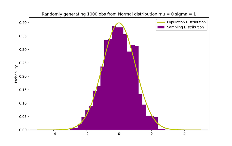
Picture Supply: The Creator

# Random Era of 1000 unbiased Regular samples
import numpy as np
mu = 0
sigma = 1
N = 1000
X = np.random.regular(mu,sigma,N)

# Inhabitants distribution
from scipy.stats import norm
x_values = np.arange(-5,5,0.01)
y_values = norm.pdf(x_values)
#Pattern histogram with Inhabitants distribution
import matplotlib.pyplot as plt
counts, bins, ignored = plt.hist(X, 30, density = True,colour="purple",label="Sampling Distribution")
plt.plot(x_values,y_values, colour="y",linewidth = 2.5,label="Inhabitants Distribution")
plt.title("Randomly producing 1000 obs from Regular distribution mu = 0 sigma = 1")
plt.ylabel("Chance")
plt.legend()
plt.present()

The Bayes Theorem or typically referred to as Bayes Regulation is arguably probably the most highly effective rule of likelihood and statistics, named after well-known English statistician and thinker, Thomas Bayes.

Picture Supply: Wikipedia

Bayes theorem is a robust likelihood legislation that brings the idea of subjectivity into the world of Statistics and Arithmetic the place every part is about info. It describes the likelihood of an occasion, based mostly on the prior data of circumstances that is perhaps associated to that occasion. As an illustration, if the chance of getting Coronavirus or Covid-19 is thought to extend with age, then Bayes Theorem permits the chance to a person of a recognized age to be decided extra precisely by conditioning it on the age than merely assuming that this particular person is widespread to the inhabitants as a complete.

The idea of conditional likelihood, which performs a central function in Bayes idea, is a measure of the likelihood of an occasion taking place, on condition that one other occasion has already occurred. Bayes theorem might be described by the next expression the place the X and Y stand for occasions X and Y, respectively:

• Pr (X|Y): the likelihood of occasion X occurring on condition that occasion or situation Y has occurred or is true
• Pr (Y|X): the likelihood of occasion Y occurring on condition that occasion or situation X has occurred or is true
• Pr (X) & Pr (Y): the chances of observing occasions X and Y, respectively

Within the case of the sooner instance, the likelihood of getting Coronavirus (occasion X) conditional on being at a sure age is Pr (X|Y), which is the same as the likelihood of being at a sure age given one obtained a Coronavirus, Pr (Y|X), multiplied with the likelihood of getting a Coronavirus, Pr (X), divided to the likelihood of being at a sure age., Pr (Y).

Earlier, the idea of causation between variables was launched, which occurs when a variable has a direct affect on one other variable. When the connection between two variables is linear, then Linear Regression is a statistical technique that may assist to mannequin the affect of a unit change in a variable, the unbiased variable on the values of one other variable, the dependent variable.

Dependent variables are sometimes called response variables or defined variables, whereas unbiased variables are sometimes called regressors or explanatory variables. When the Linear Regression mannequin relies on a single unbiased variable, then the mannequin is named Easy Linear Regression and when the mannequin relies on a number of unbiased variables, it’s known as A number of Linear Regression. Easy Linear Regression might be described by the next expression:

the place Y is the dependent variable, X is the unbiased variable which is a part of the information, ?0 is the intercept which is unknown and fixed, ?1 is the slope coefficient or a parameter akin to the variable X which is unknown and fixed as nicely. Lastly, u is the error time period that the mannequin makes when estimating the Y values. The principle thought behind linear regression is to seek out the best-fitting straight line, the regression line, via a set of paired ( X, Y ) information. One instance of the Linear Regression utility is modeling the affect of Flipper Size on penguins’ Physique Mass, which is visualized beneath.

Picture Supply: The Creator

# R code for the graph
set up.packages("ggplot2")
set up.packages("palmerpenguins")
library(palmerpenguins)
library(ggplot2)
View(information(penguins))
ggplot(information = penguins, aes(x = flipper_length_mm,y = body_mass_g))+
  geom_smooth(technique = "lm", se = FALSE, colour="purple")+
  geom_point()+
  labs(x="Flipper Size (mm)",y="Physique Mass (g)")

A number of Linear Regression with three unbiased variables might be described by the next expression:

Odd Least Squares

The peculiar least squares (OLS) is a technique for estimating the unknown parameters reminiscent of ?0 and ?1 in a linear regression mannequin. The mannequin relies on the precept of least squares that minimizes the sum of squares of the variations between the noticed dependent variable and its values predicted by the linear operate of the unbiased variable, sometimes called fitted values. This distinction between the true and predicted values of dependent variable Y is known as residual and what OLS does, is minimizing the sum of squared residuals. This optimization drawback ends in the next OLS estimates for the unknown parameters ?0 and ?1 that are often known as coefficient estimates.

As soon as these parameters of the Easy Linear Regression mannequin are estimated, the fitted values of the response variable might be computed as follows:

Commonplace Error

The residuals or the estimated error phrases might be decided as follows:

You will need to bear in mind the distinction between the error phrases and residuals. Error phrases are by no means noticed, whereas the residuals are calculated from the information. The OLS estimates the error phrases for every commentary however not the precise error time period. So, the true error variance continues to be unknown. Furthermore, these estimates are topic to sampling uncertainty. What this implies is that we are going to by no means be capable to decide the precise estimate, the true worth, of those parameters from pattern information in an empirical utility. Nevertheless, we are able to estimate it by calculating the pattern residual variance through the use of the residuals as follows.

This estimate for the variance of pattern residuals helps to estimate the variance of the estimated parameters which is commonly expressed as follows:

The squared root of this variance time period is named the usual error of the estimate which is a key element in assessing the accuracy of the parameter estimates. It’s used to calculating take a look at statistics and confidence intervals. The usual error might be expressed as follows:

You will need to bear in mind the distinction between the error phrases and residuals. Error phrases are by no means noticed, whereas the residuals are calculated from the information.

OLS Assumptions

OLS estimation technique makes the next assumption which must be happy to get dependable prediction outcomes:

A1: Linearity assumption states that the mannequin is linear in parameters.

A2: Random Pattern assumption states that each one observations within the pattern are randomly chosen.

A3: Exogeneity assumption states that unbiased variables are uncorrelated with the error phrases.

A4: Homoskedasticity assumption states that the variance of all error phrases is fixed.

A5: No Good Multi-Collinearity assumption states that not one of the unbiased variables is fixed and there are not any precise linear relationships between the unbiased variables.

def runOLS(Y,X):

   # OLS esyimation Y = Xb + e --> beta_hat = (X'X)^-1(X'Y)
   beta_hat = np.dot(np.linalg.inv(np.dot(np.transpose(X), X)), np.dot(np.transpose(X), Y))

   # OLS prediction
   Y_hat = np.dot(X,beta_hat)
   residuals = Y-Y_hat
   RSS = np.sum(np.sq.(residuals))
   sigma_squared_hat = RSS/(N-2)
   TSS = np.sum(np.sq.(Y-np.repeat(Y.imply(),len(Y))))
   MSE = sigma_squared_hat
   RMSE = np.sqrt(MSE)
   R_squared = (TSS-RSS)/TSS

   # Commonplace error of estimates:sq. root of estimate's variance
   var_beta_hat = np.linalg.inv(np.dot(np.transpose(X),X))*sigma_squared_hat
   
   SE = []
   t_stats = []
   p_values = []
   CI_s = []
   
   for i in vary(len(beta)):
       #normal errors
       SE_i = np.sqrt(var_beta_hat[i,i])
       SE.append(np.spherical(SE_i,3))

        #t-statistics
        t_stat = np.spherical(beta_hat[i,0]/SE_i,3)
        t_stats.append(t_stat)

        #p-value of t-stat p[|t_stat| >= t-treshhold two sided] 
        p_value = t.sf(np.abs(t_stat),N-2) * 2
        p_values.append(np.spherical(p_value,3))

        #Confidence intervals = beta_hat -+ margin_of_error
        t_critical = t.ppf(q =1-0.05/2, df = N-2)
        margin_of_error = t_critical*SE_i
        CI = [np.round(beta_hat[i,0]-margin_of_error,3), np.spherical(beta_hat[i,0]+margin_of_error,3)]
        CI_s.append(CI)
        return(beta_hat, SE, t_stats, p_values,CI_s, 
               MSE, RMSE, R_squared)

Underneath the belief that the OLS standards A1 — A5 are happy, the OLS estimators of coefficients β0 and β1 are BLUE and Constant.

Gauss-Markov theorem

This theorem highlights the properties of OLS estimates the place the time period BLUE stands for Finest Linear Unbiased Estimator.

Bias

The bias of an estimator is the distinction between its anticipated worth and the true worth of the parameter being estimated and might be expressed as follows:

Once we state that the estimator is unbiased what we imply is that the bias is the same as zero, which means that the anticipated worth of the estimator is the same as the true parameter worth, that’s:

Unbiasedness doesn’t assure that the obtained estimate with any specific pattern is equal or near ?. What it means is that, if one repeatedly attracts random samples from the inhabitants after which computes the estimate every time, then the typical of those estimates could be equal or very near β.

Effectivity

The time period Finest within the Gauss-Markov theorem pertains to the variance of the estimator and is known as effectivity. A parameter can have a number of estimators however the one with the bottom variance is named environment friendly.

Consistency

The time period consistency goes hand in hand with the phrases pattern dimension and convergence. If the estimator converges to the true parameter because the pattern dimension turns into very massive, then this estimator is alleged to be constant, that’s:

Underneath the belief that the OLS standards A1 — A5 are happy, the OLS estimators of coefficients β0 and β1 are BLUE and Constant.
Gauss-Markov Theorem

All these properties maintain for OLS estimates as summarized within the Gauss-Markov theorem. In different phrases, OLS estimates have the smallest variance, they’re unbiased, linear in parameters, and are constant. These properties might be mathematically confirmed through the use of the OLS assumptions made earlier.

The Confidence Interval is the vary that incorporates the true inhabitants parameter with a sure pre-specified likelihood, known as the confidence stage of the experiment, and it’s obtained through the use of the pattern outcomes and the margin of error.

Margin of Error

The margin of error is the distinction between the pattern outcomes and based mostly on what the end result would have been if one had used the complete inhabitants.

Confidence Stage

The Confidence Stage describes the extent of certainty within the experimental outcomes. For instance, a 95% confidence stage signifies that if one had been to carry out the identical experiment repeatedly for 100 occasions, then 95 of these 100 trials would result in related outcomes. Observe that the boldness stage is outlined earlier than the beginning of the experiment as a result of it’ll have an effect on how massive the margin of error might be on the finish of the experiment.

Confidence Interval for OLS Estimates

Because it was talked about earlier, the OLS estimates of the Easy Linear Regression, the estimates for intercept ?0 and slope coefficient ?1, are topic to sampling uncertainty. Nevertheless, we are able to assemble CI’s for these parameters which can include the true worth of those parameters in 95% of all samples. That’s, 95% confidence interval for ? might be interpreted as follows:

• The arrogance interval is the set of values for which a speculation take a look at can’t be rejected to the extent of 5%.
• The arrogance interval has a 95% probability to include the true worth of ?.

95% confidence interval of OLS estimates might be constructed as follows:

which relies on the parameter estimate, the usual error of that estimate, and the worth 1.96 representing the margin of error akin to the 5% rejection rule. This worth is decided utilizing the Normal Distribution table, which might be mentioned in a while on this article. In the meantime, the next determine illustrates the concept of 95% CI:

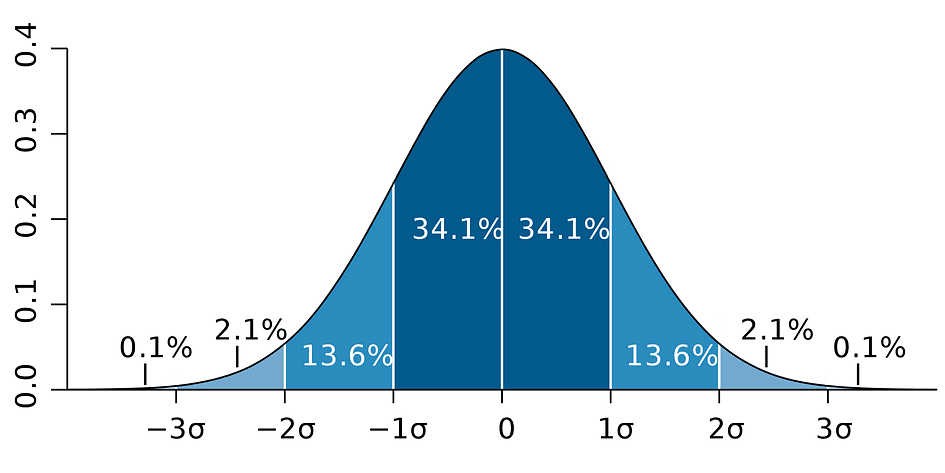
Picture Supply: Wikipedia

Observe that the boldness interval depends upon the pattern dimension as nicely, on condition that it’s calculated utilizing the usual error which relies on pattern dimension.

The arrogance stage is outlined earlier than the beginning of the experiment as a result of it’ll have an effect on how massive the margin of error might be on the finish of the experiment.

Testing a speculation in Statistics is a strategy to take a look at the outcomes of an experiment or survey to find out how significant they the outcomes are. Principally, one is testing whether or not the obtained outcomes are legitimate by determining the chances that the outcomes have occurred by probability. If it’s the letter, then the outcomes are usually not dependable and neither is the experiment. Speculation Testing is a part of the Statistical Inference.

Null and Various Speculation

Firstly, that you must decide the thesis you want to take a look at, then that you must formulate the Null Speculation and the Various Speculation. The take a look at can have two potential outcomes and based mostly on the statistical outcomes you possibly can both reject the said speculation or settle for it. As a rule of thumb, statisticians are inclined to put the model or formulation of the speculation underneath the Null Speculation that that must be rejected, whereas the suitable and desired model is said underneath the Various Speculation.

Statistical significance

Let’s take a look at the sooner talked about instance the place the Linear Regression mannequin was used to investigating whether or not a penguins’ Flipper Size, the unbiased variable, has an affect on Physique Mass, the dependent variable. We will formulate this mannequin with the next statistical expression:

Then, as soon as the OLS estimates of the coefficients are estimated, we are able to formulate the next Null and Various Speculation to check whether or not the Flipper Size has a statistically important affect on the Physique Mass:

the place H0 and H1 characterize Null Speculation and Various Speculation, respectively. Rejecting the Null Speculation would imply {that a} one-unit enhance in Flipper Size has a direct affect on the Physique Mass. On condition that the parameter estimate of ?1 is describing this affect of the unbiased variable, Flipper Size, on the dependent variable, Physique Mass. This speculation might be reformulated as follows:

the place H0 states that the parameter estimate of ?1 is the same as 0, that’s Flipper Size impact on Physique Mass is statistically insignificant whereas H0 states that the parameter estimate of ?1 is just not equal to 0 suggesting that Flipper Size impact on Physique Mass is statistically important.

Sort I and Sort II Errors

When performing Statistical Speculation Testing one wants to contemplate two conceptual sorts of errors: Sort I error and Sort II error. The Sort I error happens when the Null is wrongly rejected whereas the Sort II error happens when the Null Speculation is wrongly not rejected. A confusion matrix may help to obviously visualize the severity of those two sorts of errors.

As a rule of thumb, statisticians are inclined to put the model the speculation underneath the Null Speculation that that must be rejected, whereas the suitable and desired model is said underneath the Various Speculation.

As soon as the Null and the Various Hypotheses are said and the take a look at assumptions are outlined, the following step is to find out which statistical take a look at is acceptable and to calculate the take a look at statistic. Whether or not or to not reject or not reject the Null might be decided by evaluating the take a look at statistic with the crucial worth. This comparability exhibits whether or not or not the noticed take a look at statistic is extra excessive than the outlined crucial worth and it will possibly have two potential outcomes:

• The take a look at statistic is extra excessive than the crucial worth ? the null speculation might be rejected
• The take a look at statistic is just not as excessive because the crucial worth ? the null speculation can’t be rejected

The crucial worth relies on a prespecified significance stage ? (normally chosen to be equal to five%) and the kind of likelihood distribution the take a look at statistic follows. The crucial worth divides the realm underneath this likelihood distribution curve into the rejection area(s) and non-rejection area. There are quite a few statistical exams used to check varied hypotheses. Examples of Statistical exams are Student’s t-test, F-test, Chi-squared test, Durbin-Hausman-Wu Endogeneity test, White Heteroskedasticity test. On this article, we’ll take a look at two of those statistical exams.

The Sort I error happens when the Null is wrongly rejected whereas the Sort II error happens when the Null Speculation is wrongly not rejected.

Pupil’s t-test

One of many easiest and hottest statistical exams is the Pupil’s t-test. which can be utilized for testing varied hypotheses particularly when coping with a speculation the place the principle space of curiosity is to seek out proof for the statistically important impact of a single variable. The take a look at statistics of the t-test follows Student’s t distribution and might be decided as follows:

the place h0 within the nominator is the worth towards which the parameter estimate is being examined. So, the t-test statistics are equal to the parameter estimate minus the hypothesized worth divided by the usual error of the coefficient estimate. Within the earlier said speculation, the place we wished to check whether or not Flipper Size has a statistically important affect on Physique Mass or not. This take a look at might be carried out utilizing a t-test and the h0 is in that case equal to the 0 for the reason that slope coefficient estimate is examined towards worth 0.

There are two variations of the t-test: a two-sided t-test and a one-sided t-test. Whether or not you want the previous or the latter model of the take a look at relies upon fully on the speculation that you just need to take a look at.

The 2-sided or two-tailed t-test can be utilized when the speculation is testing equal versus not equal relationship underneath the Null and Various Hypotheses that’s much like the next instance:

The 2-sided t-test has two rejection areas as visualized within the determine beneath:

Picture Supply: Hartmann, K., Krois, J., Waske, B. (2018): E-Learning Project SOGA: Statistics and Geospatial Data Analysis. Department of Earth Sciences, Freie Universitaet Berlin

On this model of the t-test, the Null is rejected if the calculated t-statistics is both too small or too massive.

Right here, the take a look at statistics are in comparison with the crucial values based mostly on the pattern dimension and the chosen significance stage. To find out the precise worth of the cutoff level, the two-sided t-distribution table can be utilized.

The one-sided or one-tailed t-test can be utilized when the speculation is testing optimistic/detrimental versus detrimental/optimistic relationship underneath the Null and Various Hypotheses that’s much like the next examples:

One-sided t-test has a single rejection area and relying on the speculation facet the rejection area is both on the left-hand facet or the right-hand facet as visualized within the determine beneath:

Picture Supply: Hartmann, K., Krois, J., Waske, B. (2018): E-Learning Project SOGA: Statistics and Geospatial Data Analysis. Department of Earth Sciences, Freie Universitaet Berlin

On this model of the t-test, the Null is rejected if the calculated t-statistics is smaller/bigger than the crucial worth.

F-test

F-test is one other highly regarded statistical take a look at typically used to check hypotheses testing a joint statistical significance of a number of variables. That is the case while you need to take a look at whether or not a number of unbiased variables have a statistically important affect on a dependent variable. Following is an instance of a statistical speculation that may be examined utilizing the F-test:

the place the Null states that the three variables corresponding to those coefficients are collectively statistically insignificant and the Various states that these three variables are collectively statistically important. The take a look at statistics of the F-test follows F distribution and might be decided as follows:

the place the SSRrestricted is the sum of squared residuals of the restricted mannequin which is identical mannequin excluding from the information the goal variables said as insignificant underneath the Null, the SSRunrestricted is the sum of squared residuals of the unrestricted mannequin which is the mannequin that features all variables, the q represents the variety of variables which might be being collectively examined for the insignificance underneath the Null, N is the pattern dimension, and the okay is the overall variety of variables within the unrestricted mannequin. SSR values are supplied subsequent to the parameter estimates after working the OLS regression and the identical holds for the F-statistics as nicely. Following is an instance of MLR mannequin output the place the SSR and F-statistics values are marked.

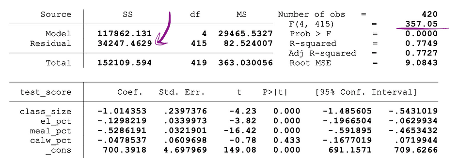
Picture Supply: Stock and Whatson

F-test has a single rejection area as visualized beneath:

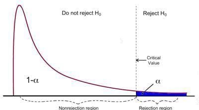
Picture Supply: U of Michigan

If the calculated F-statistics is greater than the crucial worth, then the Null might be rejected which means that the unbiased variables are collectively statistically important. The rejection rule might be expressed as follows:

One other fast strategy to decide whether or not to reject or to help the Null Speculation is through the use of p-values. The p-value is the likelihood of the situation underneath the Null occurring. Acknowledged in a different way, the p-value is the likelihood, assuming the null speculation is true, of observing a end result at the least as excessive because the take a look at statistic. The smaller the p-value, the stronger is the proof towards the Null Speculation, suggesting that it may be rejected.

The interpretation of a p-value relies on the chosen significance stage. Most frequently, 1%, 5%, or 10% significance ranges are used to interpret the p-value. So, as an alternative of utilizing the t-test and the F-test, p-values of those take a look at statistics can be utilized to check the identical hypotheses.

The next determine exhibits a pattern output of an OLS regression with two unbiased variables. On this desk, the p-value of the t-test, testing the statistical significance of class_size variable’s parameter estimate, and the p-value of the F-test, testing the joint statistical significance of the class_size, and el_pct variables parameter estimates, are underlined.

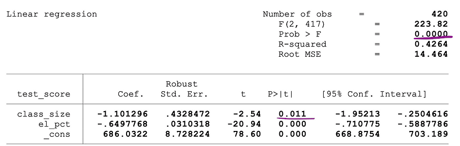
Picture Supply: Stock and Whatson

The p-value akin to the class_size variable is 0.011 and when evaluating this worth to the importance ranges 1% or 0.01 , 5% or 0.05, 10% or 0.1, then the next conclusions might be made:

• 0.011 > 0.01 ? Null of the t-test can’t be rejected at 1% significance stage
• 0.011 < 0.05 ? Null of the t-test might be rejected at 5% significance stage
• 0.011 < 0.10 ?Null of the t-test might be rejected at 10% significance stage

So, this p-value means that the coefficient of the class_size variable is statistically important at 5% and 10% significance ranges. The p-value akin to the F-test is 0.0000 and since 0 is smaller than all three cutoff values; 0.01, 0.05, 0.10, we are able to conclude that the Null of the F-test might be rejected in all three circumstances. This means that the coefficients of class_size and el_pct variables are collectively statistically important at 1%, 5%, and 10% significance ranges.

Limitation of p-values

Though, utilizing p-values has many advantages however it has additionally limitations. Particularly, the p-value depends upon each the magnitude of affiliation and the pattern dimension. If the magnitude of the impact is small and statistically insignificant, the p-value may nonetheless present a important affect as a result of the massive pattern dimension is massive. The alternative can happen as nicely, an impact might be massive, however fail to fulfill the p<0.01, 0.05, or 0.10 standards if the pattern dimension is small.

Inferential statistics makes use of pattern information to make cheap judgments in regards to the inhabitants from which the pattern information originated. It’s used to research the relationships between variables inside a pattern and make predictions about how these variables will relate to a bigger inhabitants.

Each Regulation of Giant Numbers (LLN) and Central Restrict Theorem (CLM) have a big function in Inferential statistics as a result of they present that the experimental outcomes maintain no matter what form the unique inhabitants distribution was when the information is massive sufficient. The extra information is gathered, the extra correct the statistical inferences develop into, therefore, the extra correct parameter estimates are generated.

Regulation of Giant Numbers (LLN)

Suppose X1, X2, . . . , Xn are all unbiased random variables with the identical underlying distribution, additionally referred to as unbiased identically-distributed or i.i.d, the place all X’s have the identical imply ? and normal deviation ?. Because the pattern dimension grows, the likelihood that the typical of all X’s is the same as the imply ? is the same as 1. The Regulation of Giant Numbers might be summarized as follows:

Central Restrict Theorem (CLM)

Suppose X1, X2, . . . , Xn are all unbiased random variables with the identical underlying distribution, additionally referred to as unbiased identically-distributed or i.i.d, the place all X’s have the identical imply ? and normal deviation ?. Because the pattern dimension grows, the likelihood distribution of X converges within the distribution in Regular distribution with imply ? and variance ?-squared. The Central Restrict Theorem might be summarized as follows:

Acknowledged in a different way, when you could have a inhabitants with imply ? and normal deviation ? and you’re taking sufficiently massive random samples from that inhabitants with substitute, then the distribution of the pattern means might be roughly usually distributed.

Dimensionality discount is the transformation of knowledge from a high-dimensional house right into a low-dimensional house such that this low-dimensional illustration of the information nonetheless incorporates the significant properties of the unique information as a lot as potential.

With the rise in recognition in Large Information, the demand for these dimensionality discount strategies, lowering the quantity of pointless information and options, elevated as nicely. Examples of fashionable dimensionality discount strategies are Principle Component Analysis, Factor Analysis, Canonical Correlation, Random Forest.

Precept Element Evaluation (PCA)

Principal Element Evaluation or PCA is a dimensionality discount method that could be very typically used to cut back the dimensionality of huge information units, by reworking a big set of variables right into a smaller set that also incorporates a lot of the data or the variation within the authentic massive dataset.

Let’s assume we now have an information X with p variables; X1, X2, …., Xp with eigenvectors e1, …, ep, and eigenvalues ?1,…, ?p. Eigenvalues present the variance defined by a selected information subject out of the overall variance. The thought behind PCA is to create new (unbiased) variables, referred to as Principal Parts, which might be a linear mixture of the present variable. The ith principal element might be expressed as follows:

Then utilizing Elbow Rule or Kaiser Rule, you possibly can decide the variety of principal parts that optimally summarize the information with out shedding an excessive amount of data. Additionally it is essential to have a look at the proportion of whole variation (PRTV) that’s defined by every principal element to determine whether or not it’s helpful to incorporate or to exclude it. PRTV for the ith principal element might be calculated utilizing eigenvalues as follows:

Elbow Rule

The elbow rule or the elbow technique is a heuristic strategy that’s used to find out the variety of optimum principal parts from the PCA outcomes. The thought behind this technique is to plot the defined variation as a operate of the variety of parts and choose the elbow of the curve because the variety of optimum principal parts. Following is an instance of such a scatter plot the place the PRTV (Y-axis) is plotted on the variety of principal parts (X-axis). The elbow corresponds to the X-axis worth 2, which means that the variety of optimum principal parts is 2.

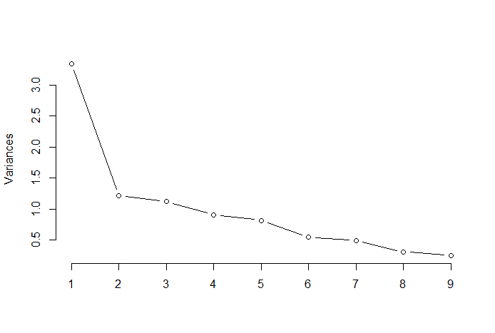
Picture Supply: Multivariate Statistics Github

Issue Evaluation (FA)

Issue evaluation or FA is one other statistical technique for dimensionality discount. It is likely one of the mostly used inter-dependency strategies and is used when the related set of variables exhibits a scientific inter-dependence and the target is to seek out out the latent components that create a commonality. Let’s assume we now have an information X with p variables; X1, X2, …., Xp. FA mannequin might be expressed as follows:

the place X is a [p x N] matrix of p variables and N observations, µ is [p x N] inhabitants imply matrix, A is [p x k] widespread issue loadings matrix, F [k x N] is the matrix of widespread components and u [pxN] is the matrix of particular components. So, put it in a different way, an element mannequin is as a collection of a number of regressions, predicting every of the variables Xi from the values of the unobservable widespread components fi:

Every variable has okay of its personal widespread components, and these are associated to the observations by way of issue loading matrix for a single commentary as follows: In issue evaluation, the components are calculated to maximize between-group variance whereas minimizing in-group variance. They’re components as a result of they group the underlying variables. Not like the PCA, in FA the information must be normalized, on condition that FA assumes that the dataset follows Regular Distribution.

 
 
Tatev Karen Aslanyan is an skilled full-stack information scientist with a give attention to Machine Studying and AI. She can be the co-founder of LunarTech, a web based tech instructional platform, and the creator of The Final Information Science Bootcamp.Tatev Karen, with Bachelor and Masters in Econometrics and Administration Science, has grown within the subject of Machine Studying and AI, specializing in Recommender Programs and NLP, supported by her scientific analysis and revealed papers. Following 5 years of instructing, Tatev is now channeling her ardour into LunarTech, serving to form the way forward for information science.

 
Original. Reposted with permission.