How one can Deal with Outliers in Dataset with Pandas


Picture by Creator
Outliers are irregular observations that differ considerably from the remainder of your information. They might happen resulting from experimentation error, measurement error, or just that variability is current inside the information itself. These outliers can severely affect your mannequin’s efficiency, resulting in biased outcomes – very like how a prime performer in relative grading at universities can increase the typical and have an effect on the grading standards. Dealing with outliers is an important a part of the info cleansing process.
On this article, I am going to share how one can spot outliers and other ways to take care of them in your dataset.
Detecting Outliers
There are a number of strategies used to detect outliers. If I had been to categorise them, right here is the way it appears to be like:
- Visualization-Based mostly Strategies: Plotting scatter plots or field plots to see information distribution and examine it for irregular information factors.
- Statistics-Based mostly Strategies: These approaches contain z scores and IQR (Interquartile Vary) which supply reliability however could also be much less intuitive.
I will not cowl these strategies extensively to remain targeted, on the subject. Nonetheless, I am going to embrace some references on the finish, for exploration. We’ll use the IQR technique in our instance. Right here is how this technique works:
IQR (Interquartile Vary) = Q3 (seventy fifth percentile) – Q1 (twenty fifth percentile)
The IQR technique states that any information factors under Q1 – 1.5 * IQR or above Q3 + 1.5 * IQR are marked as outliers. Let’s generate some random information factors and detect the outliers utilizing this technique.
Make the required imports and generate the random information utilizing np.random:
import pandas as pd
import numpy as np
import matplotlib.pyplot as plt
import seaborn as sns

# Generate random information
np.random.seed(42)
information = pd.DataFrame({
    'worth': np.random.regular(0, 1, 1000)
})
Detect the outliers from the dataset utilizing the IQR Technique:
# Operate to detect outliers utilizing IQR
def detect_outliers_iqr(information):
    Q1 = information.quantile(0.25)
    Q3 = information.quantile(0.75)
    IQR = Q3 - Q1
    lower_bound = Q1 - 1.5 * IQR
    upper_bound = Q3 + 1.5 * IQR
    return (information  upper_bound)

# Detect outliers
outliers = detect_outliers_iqr(information['value'])

print(f"Variety of outliers detected: {sum(outliers)}")
Output ⇒ Variety of outliers detected: 8
Visualize the dataset utilizing scatter and field plots to see the way it appears to be like
# Visualize the info with outliers utilizing scatter plot and field plot
fig, (ax1, ax2) = plt.subplots(1, 2, figsize=(15, 6))

# Scatter plot
ax1.scatter(vary(len(information)), information['value'], c=['blue' if not x else 'red' for x in outliers])
ax1.set_title('Dataset with Outliers Highlighted (Scatter Plot)')
ax1.set_xlabel('Index')
ax1.set_ylabel('Worth')

# Field plot
sns.boxplot(x=information['value'], ax=ax2)
ax2.set_title('Dataset with Outliers (Field Plot)')
ax2.set_xlabel('Worth')

plt.tight_layout()
plt.present()
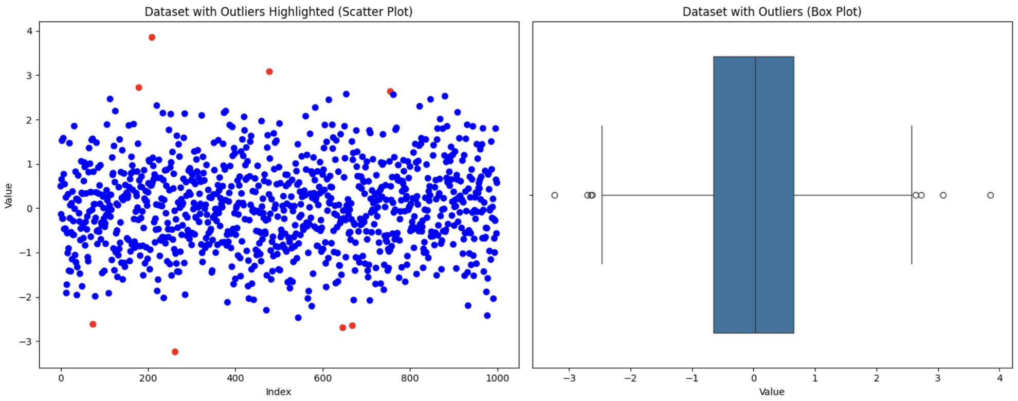
Unique Dataset
Now that we now have detected the outliers, let’s talk about a number of the other ways to deal with the outliers.
Dealing with Outliers
1. Eradicating Outliers
This is without doubt one of the easiest approaches however not all the time the appropriate one. It’s good to think about sure elements. If eradicating these outliers considerably reduces your dataset dimension or in the event that they maintain helpful insights, then excluding them out of your evaluation not be probably the most favorable determination. Nonetheless, in the event that they’re resulting from measurement errors and few in quantity, then this method is appropriate. Let’s apply this method to the dataset generated above:
# Take away outliers
data_cleaned = information[~outliers]

print(f"Unique dataset dimension: {len(information)}")
print(f"Cleaned dataset dimension: {len(data_cleaned)}")

fig, (ax1, ax2) = plt.subplots(1, 2, figsize=(15, 6))

# Scatter plot
ax1.scatter(vary(len(data_cleaned)), data_cleaned['value'])
ax1.set_title('Dataset After Eradicating Outliers (Scatter Plot)')
ax1.set_xlabel('Index')
ax1.set_ylabel('Worth')

# Field plot
sns.boxplot(x=data_cleaned['value'], ax=ax2)
ax2.set_title('Dataset After Eradicating Outliers (Field Plot)')
ax2.set_xlabel('Worth')

plt.tight_layout()
plt.present()
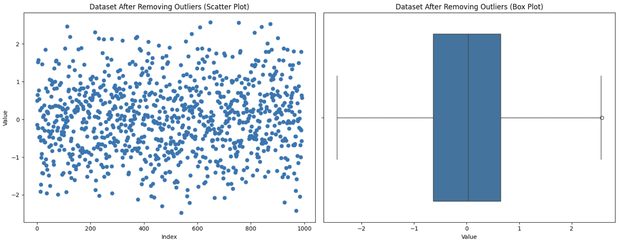
Eradicating Outliers
Discover that the distribution of the info can really be modified by eradicating outliers. In case you take away some preliminary outliers, the definition of what’s an outlier might very properly change. Due to this fact, information that will have been within the regular vary earlier than, could also be thought-about outliers beneath a brand new distribution. You possibly can see a brand new outlier with the brand new field plot.
2. Capping Outliers
This method is used when you do not need to discard your information factors however maintaining these excessive values may also affect your evaluation. So, you set a threshold for the utmost and the minimal values after which deliver the outliers inside this vary. You possibly can apply this capping to outliers or to your dataset as an entire too. Let’s apply the capping technique to our full dataset to deliver it inside the vary of the Fifth-Ninety fifth percentile. Right here is how one can execute this:
def cap_outliers(information, lower_percentile=5, upper_percentile=95):
    lower_limit = np.percentile(information, lower_percentile)
    upper_limit = np.percentile(information, upper_percentile)
    return np.clip(information, lower_limit, upper_limit)

information['value_capped'] = cap_outliers(information['value'])

fig, (ax1, ax2) = plt.subplots(1, 2, figsize=(15, 6))

# Scatter plot
ax1.scatter(vary(len(information)), information['value_capped'])
ax1.set_title('Dataset After Capping Outliers (Scatter Plot)')
ax1.set_xlabel('Index')
ax1.set_ylabel('Worth')

# Field plot
sns.boxplot(x=information['value_capped'], ax=ax2)
ax2.set_title('Dataset After Capping Outliers (Field Plot)')
ax2.set_xlabel('Worth')

plt.tight_layout()
plt.present()
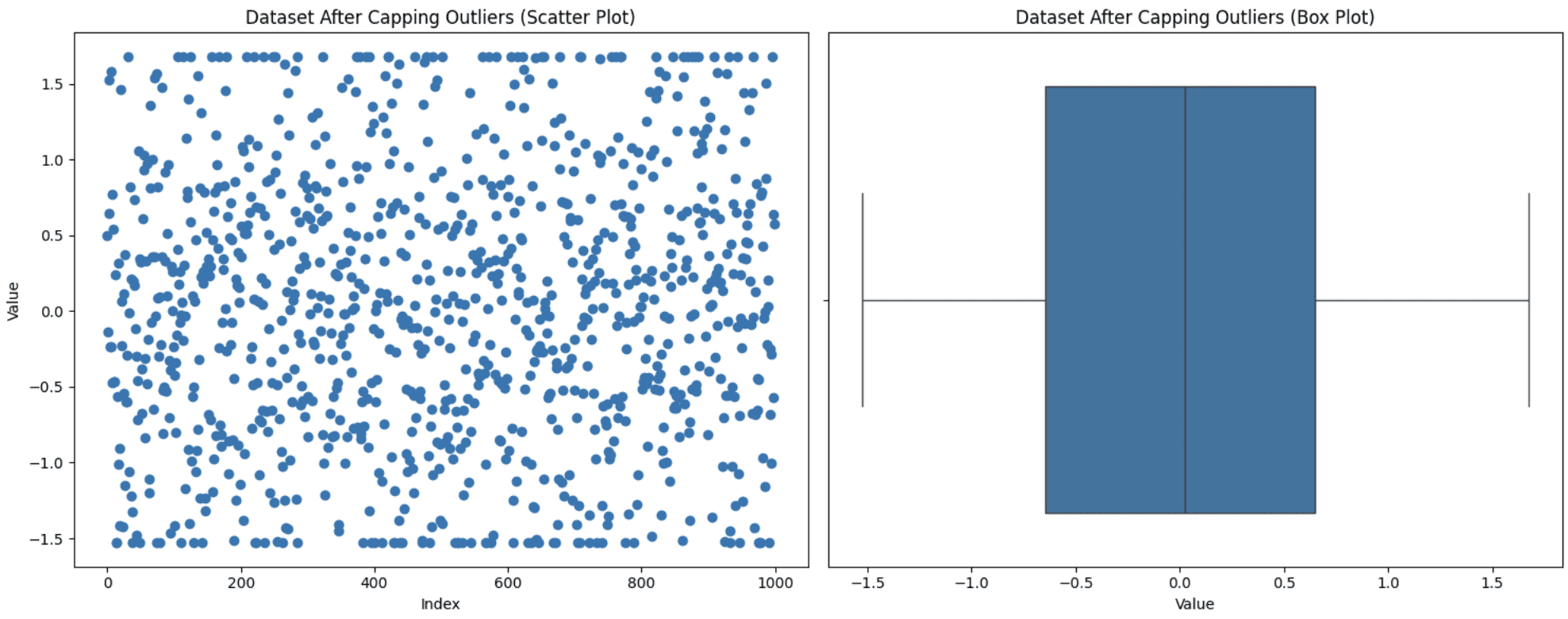
Capping Outliers
You possibly can see from the graph that the higher and decrease factors within the scatter plot seem like in a line resulting from capping.
3. Imputing Outliers
Generally eradicating values from the evaluation is not an choice as it could result in info loss, and also you additionally don’t need these values to be set to max or min like in capping. On this scenario, one other method is to substitute these values with extra significant choices like imply, median, or mode. The selection varies relying on the area of knowledge beneath statement, however be aware of not introducing biases whereas utilizing this method. Let’s exchange our outliers with the mode (probably the most steadily occurring worth) worth and see how the graph seems:
information['value_imputed'] = information['value'].copy()
median_value = information['value'].median()
information.loc[outliers, 'value_imputed'] = median_value

fig, (ax1, ax2) = plt.subplots(1, 2, figsize=(15, 6))

# Scatter plot
ax1.scatter(vary(len(information)), information['value_imputed'])
ax1.set_title('Dataset After Imputing Outliers (Scatter Plot)')
ax1.set_xlabel('Index')
ax1.set_ylabel('Worth')

# Field plot
sns.boxplot(x=information['value_imputed'], ax=ax2)
ax2.set_title('Dataset After Imputing Outliers (Field Plot)')
ax2.set_xlabel('Worth')

plt.tight_layout()
plt.present()
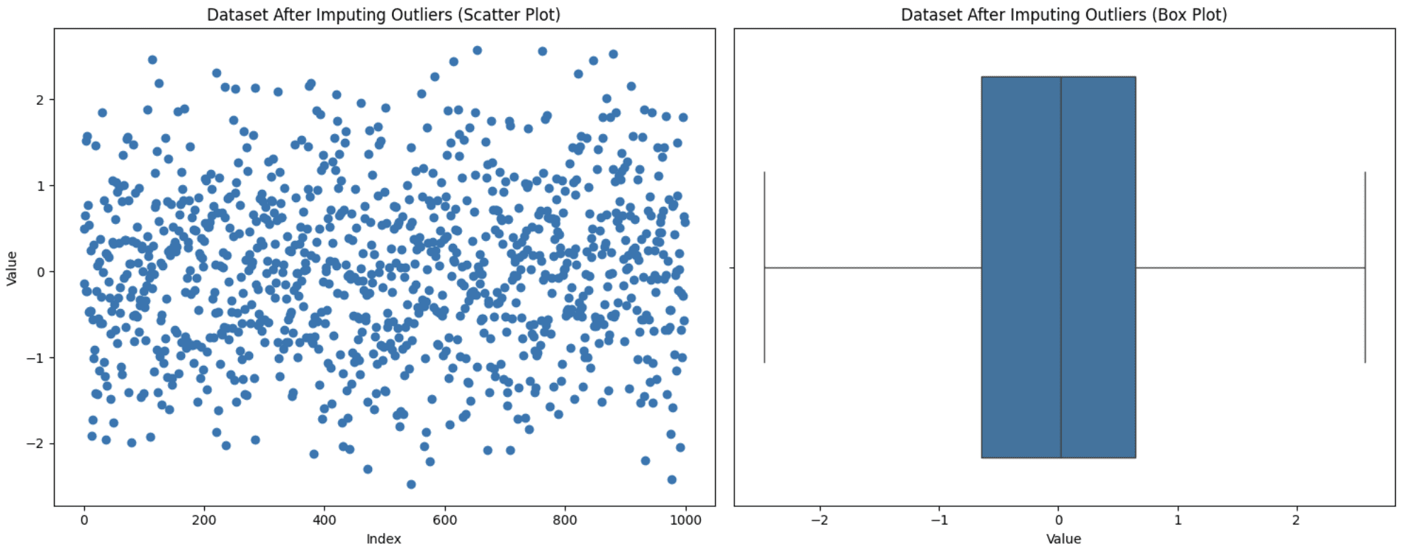
Imputing Outliers
Discover that now we have no outliers, however this does not assure that outliers shall be eliminated since after the imputation, the IQR additionally modifications. It’s good to experiment to see what suits finest in your case.
4. Making use of a Transformation
Transformation is utilized to your full dataset as an alternative of particular outliers. You mainly change the best way your information is represented to cut back the affect of the outliers. There are a number of transformation strategies like log transformation, sq. root transformation, box-cox transformation, Z-scaling, Yeo-Johnson transformation, min-max scaling, and so on. Choosing the proper transformation in your case is determined by the character of the info and your finish purpose of the evaluation. Listed below are just a few suggestions that can assist you choose the appropriate transformation approach:
- For right-skewed information: Use log, sq. root, or Field-Cox transformation. Log is even higher whenever you wish to compress small quantity values which are unfold over a big scale. Sq. root is healthier when, aside from proper skew, you desire a much less excessive transformation and in addition wish to deal with zero values, whereas Field-Cox additionally normalizes your information, which the opposite two do not.
- For left-skewed information: Replicate the info first after which apply the strategies talked about for right-skewed information.
- To stabilize variance: Use Field-Cox or Yeo-Johnson (much like Field-Cox however handles zero and unfavorable values as properly).
- For mean-centering and scaling: Use z-score standardization (customary deviation = 1).
- For range-bound scaling (mounted vary i.e., [2,5]): Use min-max scaling.
Let’s generate a right-skewed dataset and apply the log transformation to the whole information to see how this works:
import pandas as pd
import numpy as np
import matplotlib.pyplot as plt
import seaborn as sns

# Generate right-skewed information
np.random.seed(42)
information = np.random.exponential(scale=2, dimension=1000)
df = pd.DataFrame(information, columns=['value'])

# Apply Log Transformation (shifted to keep away from log(0))
df['log_value'] = np.log1p(df['value'])

fig, axes = plt.subplots(2, 2, figsize=(15, 10))

# Unique Information - Scatter Plot
axes[0, 0].scatter(vary(len(df)), df['value'], alpha=0.5)
axes[0, 0].set_title('Unique Information (Scatter Plot)')
axes[0, 0].set_xlabel('Index')
axes[0, 0].set_ylabel('Worth')

# Unique Information - Field Plot
sns.boxplot(x=df['value'], ax=axes[0, 1])
axes[0, 1].set_title('Unique Information (Field Plot)')
axes[0, 1].set_xlabel('Worth')

# Log Reworked Information - Scatter Plot
axes[1, 0].scatter(vary(len(df)), df['log_value'], alpha=0.5)
axes[1, 0].set_title('Log Reworked Information (Scatter Plot)')
axes[1, 0].set_xlabel('Index')
axes[1, 0].set_ylabel('Log(Worth)')

# Log Reworked Information - Field Plot
sns.boxplot(x=df['log_value'], ax=axes[1, 1])
axes[1, 1].set_title('Log Reworked Information (Field Plot)')
axes[1, 1].set_xlabel('Log(Worth)')

plt.tight_layout()
plt.present()

Making use of Log Transformation
You possibly can see {that a} easy transformation has dealt with a lot of the outliers itself and decreased them to only one. This reveals the facility of transformation in dealing with outliers. On this case, it’s essential to be cautious and know your information properly sufficient to decide on acceptable transformation as a result of failing to take action might trigger issues for you.
Wrapping Up
This brings us to the top of our dialogue about outliers, other ways to detect them, and learn how to deal with them. This text is a part of the pandas collection, and you’ll test different articles on my writer web page. As talked about above, listed here are some further sources so that you can examine extra about outliers:
- Outlier detection methods in Machine Learning
- Different transformations in Machine Learning
- Types Of Transformations For Better Normal Distribution
Kanwal Mehreen Kanwal is a machine studying engineer and a technical author with a profound ardour for information science and the intersection of AI with drugs. She co-authored the e-book “Maximizing Productiveness with ChatGPT”. As a Google Technology Scholar 2022 for APAC, she champions range and tutorial excellence. She’s additionally acknowledged as a Teradata Range in Tech Scholar, Mitacs Globalink Analysis Scholar, and Harvard WeCode Scholar. Kanwal is an ardent advocate for change, having based FEMCodes to empower ladies in STEM fields.