Diffusion and Denoising: Explaining Textual content-to-Picture Generative AI

The Idea of Diffusion

 
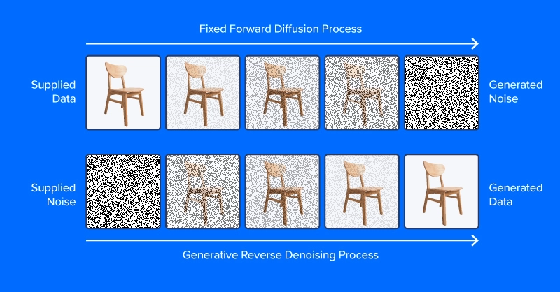
Denoising diffusion fashions are educated to drag patterns out of noise, to generate a fascinating picture. The coaching course of entails displaying mannequin examples of photos (or different information) with various ranges of noise decided in response to a noise scheduling algorithm, meaning to predict what elements of the information are noise. If profitable, the noise prediction mannequin will be capable of steadily construct up a realistic-looking picture from pure noise, subtracting increments of noise from the picture at every time step.

In contrast to the picture on the prime of this part, trendy diffusion fashions don’t predict noise from a picture with added noise, a minimum of circuitously. As an alternative, they predict noise in a latent house illustration of the picture. Latent house represents photos in a compressed set of numerical options, the output of an encoding module from a variational autoencoder, or VAE. This trick put the “latent” in latent diffusion, and vastly lowered the time and computational necessities for producing photos. As reported by the paper authors, latent diffusion hastens inference by a minimum of ~2.7X over direct diffusion and trains about 3 times quicker.

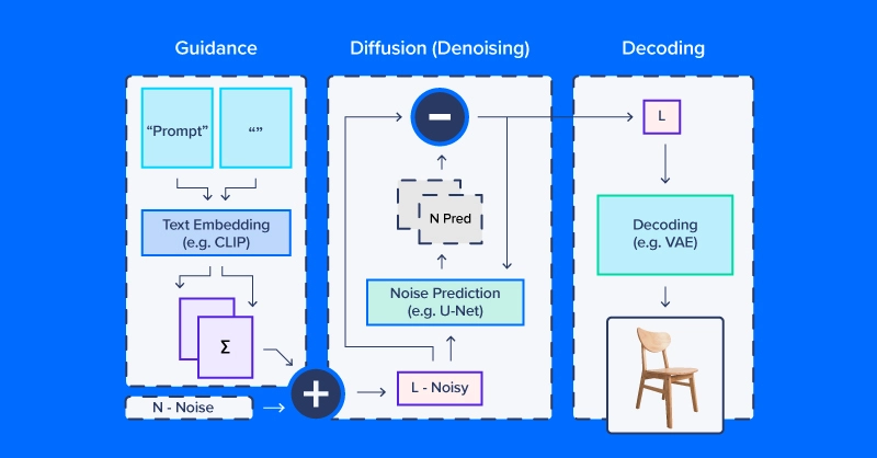
Individuals working with latent diffusion typically speak of utilizing a “diffusion mannequin,” however in reality, the diffusion course of employs a number of modules. As within the diagram above, a diffusion pipeline for text-to-image workflows usually features a textual content embedding mannequin (and its tokenizer), a denoise prediction/diffusion mannequin, and a picture decoder. One other vital a part of latent diffusion is the scheduler, which determines how the noise is scaled and up to date over a collection of “time steps” (a collection of iterative updates that steadily take away noise from latent house).

Latent Diffusion Code Instance

 
We’ll use CompVis/latent-diffusion-v1-4 for many of our examples. Textual content embedding is dealt with by a CLIPTextModel and CLIPTokenizer. Noise prediction makes use of a ‘U-Net,’ a sort of image-to-image mannequin that initially gained traction as a mannequin for purposes in biomedical photos (particularly segmentation). To generate photos from denoised latent arrays, the pipeline makes use of a variational autoencoder (VAE) for picture decoding, turning these arrays into photos.

We’ll begin by constructing our model of this pipeline from HuggingFace elements.

# native setup
virtualenv diff_env –python=python3.8
supply diff_env/bin/activate
pip set up diffusers transformers huggingface-hub
pip set up torch --index-url https://obtain.pytorch.org/whl/cu118

Be certain to verify pytorch.org to make sure the correct model to your system in the event you’re working regionally. Our imports are comparatively simple, and the code snippet beneath suffices for all the next demos.

import os
import numpy as np
import torch
from diffusers import StableDiffusionPipeline, AutoPipelineForImage2Image
from diffusers.pipelines.pipeline_utils import numpy_to_pil
from transformers import CLIPTokenizer, CLIPTextModel
from diffusers import AutoencoderKL, UNet2DConditionModel, 
       PNDMScheduler, LMSDiscreteScheduler

from PIL import Picture
import matplotlib.pyplot as plt

Now for the main points. Begin by defining picture and diffusion parameters and a immediate.

immediate = [" "]

# picture settings
top, width = 512, 512

# diffusion settings
number_inference_steps = 64
guidance_scale = 9.0
batch_size = 1

Initialize your pseudorandom quantity generator with a seed of your alternative for reproducing your outcomes.

def seed_all(seed):
    torch.manual_seed(seed)
    np.random.seed(seed)

seed_all(193)

Now we will initialize the textual content embedding mannequin, autoencoder, a U-Web, and the time step scheduler.

tokenizer = CLIPTokenizer.from_pretrained("openai/clip-vit-large-patch14")
text_encoder = CLIPTextModel.from_pretrained("openai/clip-vit-large-patch14")
vae = AutoencoderKL.from_pretrained("CompVis/stable-diffusion-v1-4", 
        subfolder="vae")
unet = UNet2DConditionModel.from_pretrained("CompVis/stable-diffusion-v1-4",
        subfolder="unet")
scheduler = PNDMScheduler()
scheduler.set_timesteps(number_inference_steps)

my_device = torch.system("cuda") if torch.cuda.is_available() else torch.system("cpu")
vae = vae.to(my_device)
text_encoder = text_encoder.to(my_device)
unet = unet.to(my_device)

Encoding the textual content immediate as an embedding requires first tokenizing the string enter. Tokenization replaces characters with integer codes equivalent to a vocabulary of semantic models, e.g. through byte pair encoding (BPE). Our pipeline embeds a null immediate (no textual content) alongside the textual immediate for our picture. This balances the diffusion course of between the supplied description and natural-appearing photos generally. We’ll see easy methods to change the relative weighting of those elements later on this article.

immediate = immediate * batch_size
tokens = tokenizer(immediate, padding="max_length",
max_length=tokenizer.model_max_length, truncation=True,
        return_tensors="pt")

empty_tokens = tokenizer([""] * batch_size, padding="max_length",
max_length=tokenizer.model_max_length, truncation=True,
        return_tensors="pt")
with torch.no_grad():
    text_embeddings = text_encoder(tokens.input_ids.to(my_device))[0]
    max_length = tokens.input_ids.form[-1]
    notext_embeddings = text_encoder(empty_tokens.input_ids.to(my_device))[0]
    text_embeddings = torch.cat([notext_embeddings, text_embeddings])

We initialize latent house as random regular noise and scale it in response to our diffusion time step scheduler.

latents = torch.randn(batch_size, unet.config.in_channels, 
        top//8, width//8)
latents = (latents * scheduler.init_noise_sigma).to(my_device)

Every part is able to go, and we will dive into the diffusion loop itself. We are able to hold observe of photos by sampling periodically all through so we will see how noise is steadily decreased.

photos = []
display_every = number_inference_steps // 8

# diffusion loop
for step_idx, timestep in enumerate(scheduler.timesteps):
    with torch.no_grad():
        # concatenate latents, to run null/textual content immediate in parallel.
        model_in = torch.cat([latents] * 2)
        model_in = scheduler.scale_model_input(model_in,
                timestep).to(my_device)
        predicted_noise = unet(model_in, timestep, 
                encoder_hidden_states=text_embeddings).pattern
        # pnu - empty immediate unconditioned noise prediction
        # pnc - textual content immediate conditioned noise prediction
        pnu, pnc = predicted_noise.chunk(2)
        # weight noise predictions in response to steerage scale
        predicted_noise = pnu + guidance_scale * (pnc - pnu)
        # replace the latents
        latents = scheduler.step(predicted_noise, 
                timestep, latents).prev_sample
        # Periodically log photos and print progress throughout diffusion
        if step_idx % display_every == 0
                or step_idx + 1 == len(scheduler.timesteps):
           picture = vae.decode(latents / 0.18215).pattern[0]
           picture = ((picture / 2.) + 0.5).cpu().permute(1,2,0).numpy()
           picture = np.clip(picture, 0, 1.0)
           photos.prolong(numpy_to_pil(picture))
           print(f"step {step_idx}/{number_inference_steps}: {timestep:.4f}")

On the finish of the diffusion course of, we’ve an honest rendering of what you needed to generate. Subsequent, we’ll go over extra strategies for better management. As we’ve already made our diffusion pipeline, we will use the streamlined diffusion pipeline from HuggingFace for the remainder of our examples.

Controlling the Diffusion Pipeline

We’ll use a set of helper features on this part:

def seed_all(seed):
    torch.manual_seed(seed)
    np.random.seed(seed)

def grid_show(photos, rows=3):
    number_images = len(photos)
    top, width = photos[0].dimension
    columns = int(np.ceil(number_images / rows))
    grid = np.zeros((top*rows,width*columns,3))
    for ii, picture in enumerate(photos):
        grid[ii//columns*height:ii//columns*height+height, 
                ii%columns*width:ii%columns*width+width] = picture
        fig, ax = plt.subplots(1,1, figsize=(3*columns, 3*rows))
        ax.imshow(grid / grid.max())
    return grid, fig, ax

def callback_stash_latents(ii, tt, latents):
    # tailored from fastai/diffusion-nbs/stable_diffusion.ipynb
    latents = 1.0 / 0.18215 * latents
    picture = pipe.vae.decode(latents).pattern[0]
    picture = (picture / 2. + 0.5).cpu().permute(1,2,0).numpy()
    picture = np.clip(picture, 0, 1.0)
    photos.prolong(pipe.numpy_to_pil(picture))

my_seed = 193

We’ll begin with probably the most well-known and easy software of diffusion fashions: picture technology from textual prompts, often called text-to-image technology. The mannequin we’ll use was launched into the wild (of the Hugging Face Hub) by the tutorial lab that revealed the latent diffusion paper. Hugging Face coordinates workflows like latent diffusion through the handy pipeline API. We wish to outline what system and what floating level to calculate based mostly on if we’ve or wouldn’t have a GPU.

if (1):
    #Run CompVis/stable-diffusion-v1-4 on GPU
    pipe_name = "CompVis/stable-diffusion-v1-4"
    my_dtype = torch.float16
    my_device = torch.system("cuda")
    my_variant = "fp16"
    pipe = StableDiffusionPipeline.from_pretrained(pipe_name,
    safety_checker=None, variant=my_variant,
        torch_dtype=my_dtype).to(my_device)
else:
    #Run CompVis/stable-diffusion-v1-4 on CPU
    pipe_name = "CompVis/stable-diffusion-v1-4"
    my_dtype = torch.float32
    my_device = torch.system("cpu")
    pipe = StableDiffusionPipeline.from_pretrained(pipe_name, 
            torch_dtype=my_dtype).to(my_device)

Steerage Scale

For those who use a really uncommon textual content immediate (very not like these within the dataset), it’s potential to finish up in a less-traveled a part of latent house. The null immediate embedding supplies a steadiness and mixing the 2 in response to guidance_scale means that you can commerce off the specificity of your immediate towards widespread picture traits.

guidance_images = []
for steerage in [0.25, 0.5, 1.0, 2.0, 4.0, 6.0, 8.0, 10.0, 20.0]:
    seed_all(my_seed)
    my_output = pipe(my_prompt, num_inference_steps=50, 
    num_images_per_prompt=1, guidance_scale=steerage)
    guidance_images.append(my_output.photos[0])
    for ii, img in enumerate(my_output.photos):
        img.save(f"prompt_{my_seed}_g{int(steerage*2)}_{ii}.jpg")

temp = grid_show(guidance_images, rows=3)
plt.savefig("prompt_guidance.jpg")
plt.present()

Since we generated the immediate utilizing the 9 steerage coefficients, you’ll be able to plot the immediate and think about how the diffusion developed. The default steerage coefficient is 0.75 so on the seventh picture could be the default picture output.

Damaging Prompts

Generally latent diffusion actually “desires” to supply a picture that doesn’t match your intentions. In these eventualities, you need to use a damaging immediate to push the diffusion course of away from undesirable outputs. For instance, we may use a damaging immediate to make our Martian astronaut diffusion outputs rather less human.

my_prompt = " "
my_negative_prompt = " "

output_x = pipe(my_prompt, num_inference_steps=50, num_images_per_prompt=9, 
        negative_prompt=my_negative_prompt)

temp = grid_show(output_x)
plt.present()

You must obtain outputs that comply with your immediate whereas avoiding outputting the issues described in your damaging immediate.

Picture Variation

Textual content-to-image technology from scratch will not be the one software for diffusion pipelines. Really, diffusion is well-suited for picture modification, ranging from an preliminary picture. We’ll use a barely totally different pipeline and pre-trained mannequin tuned for image-to-image diffusion.

pipe_img2img = AutoPipelineForImage2Image.from_pretrained(

        "runwayml/stable-diffusion-v1-5", safety_checker=None,

torch_dtype=my_dtype, use_safetensors=True).to(my_device)

One software of this strategy is to generate variations on a theme. An idea artist may use this method to rapidly iterate totally different concepts for illustrating an exoplanet based mostly on the newest analysis.

We’ll first obtain a public area artist’s idea of planet 1e within the TRAPPIST system (credit: NASA/JPL-Caltech).
Then, after downscaling to take away particulars, we’ll use a diffusion pipeline to make a number of totally different variations of the exoplanet TRAPPIST-1e.

url = 
"https://add.wikimedia.org/wikipedia/commons/thumb/3/38/TRAPPIST-1e_artist_impression_2018.png/600px-TRAPPIST-1e_artist_impression_2018.png"
img_path = url.break up("https://www.kdnuggets.com/")[-1]
if not (os.path.exists("600px-TRAPPIST-1e_artist_impression_2018.png")):
    os.system(f"wget      '{url}'")
    init_image = Picture.open(img_path)

seed_all(my_seed)

trappist_prompt = "Artist's impression of TRAPPIST-1e"
                  "massive Earth-like water-world exoplanet with oceans,"
                  "NASA, artist idea, sensible, detailed, intricate"

my_negative_prompt = "cartoon, sketch, orbiting moon"

my_output_trappist1e = pipe_img2img(immediate=trappist_prompt, num_images_per_prompt=9, 
     picture=init_image, negative_prompt=my_negative_prompt, guidance_scale=6.0)

grid_show(my_output_trappist1e.photos)
plt.present()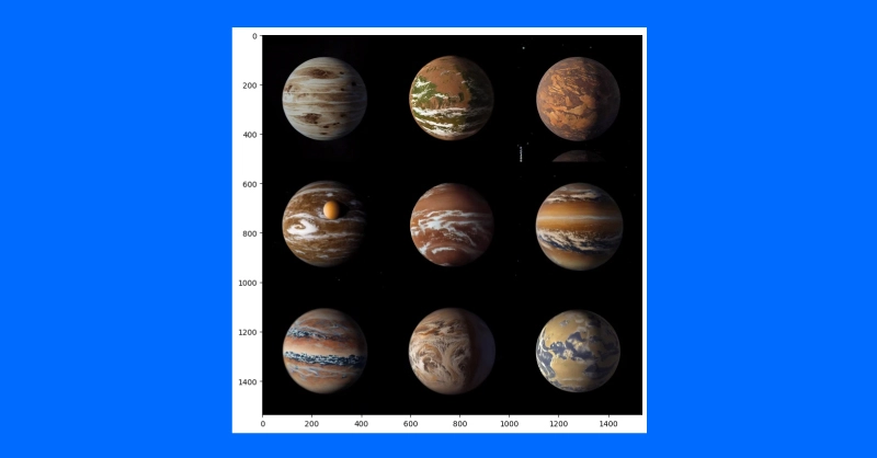

By feeding the mannequin an instance preliminary picture, we will generate comparable photos. You can even use a text-guided image-to-image pipeline to vary the type of a picture by growing the steerage, including damaging prompts and extra comparable to “non-realistic” or “watercolor” or “paper sketch.” Your mile could differ and adjusting your prompts would be the best solution to discover the correct picture you wish to create.

Conclusions

 
Regardless of the discourse behind diffusion programs and imitating human generated artwork, diffusion fashions produce other extra impactful functions. It has been applied to protein folding prediction for protein design and drug improvement. Textual content-to-video can also be an active area of research and is obtainable by a number of firms (e.g. Stability AI, Google). Diffusion can also be an emerging approach for text-to-speech purposes.

It’s clear that the diffusion course of is taking a central position within the evolution of AI and the interplay of know-how with the worldwide human setting. Whereas the intricacies of copyright, different mental property legal guidelines, and the impression on human artwork and science are evident in each constructive and damaging methods. However what is actually a constructive is the unprecedented functionality AI has to know language and generate photos. It was AlexNet that had computer systems analyze a picture and output textual content, and solely now computer systems can analyze textual prompts and output coherent photos.

 
Original. Republished with permission.
 
 

Kevin Vu manages Exxact Corp blog and works with lots of its proficient authors who write about totally different points of Deep Studying.