Binary Classification. Unpacking the Actual Significance and… | by gabriel costa
Unpacking the Actual Significance and Limitations of Conventional Metrics
The work of classification might be seen as a method of summarizing the complexity of buildings into finite courses, and it’s usually helpful to make life boring sufficient that we are able to scale back such buildings into two single sorts. These labels might have apparent interpretations, as within the case the place we differentiate Statisticians from Knowledge Scientists (presumably utilizing earnings as a singular believable function), or they might even be a suffocating try to cut back experimental proof into sentences, rejecting or not a null speculation. Embracing the metalanguage, we attribute a classification label to the work itself of sum up stuff into two differing types: Binary Classification. This work is an try at a deeper description of this particular label, bringing a probabilistic interpretation of what the choice course of means and the metrics we use to judge our outcomes.
Once we attempt to describe and differentiate an object, we goal to search out particular traits that spotlight its uniqueness. It’s anticipated that for a lot of attributes this distinction shouldn’t be constantly correct throughout a inhabitants.
For an regular downside of two courses with totally different n options (V1, … Vn), we are able to se how these function values distribute and attempt to make conclusions from them:

If the duty had been to make use of a kind of options to information our choice course of, the technique of deciding, given a person’s v_n worth,
it will be intuitive to foretell the category with the very best frequency (or highest likelihood, if our histograms are good estimators of our distributions). As an example, if v4 measure for a particular person had been larger than 5, then it will be very doubtless that it’s a constructive.
Nevertheless, we are able to do greater than that, and take benefit totally different options, in order that we are able to synthesize the data right into a single distribution. That is the job of the rating operate S(x). The rating operate will do a regression to squeeze the function distributions in a single distinctive distribution P(s, y), which might be conditioned to every of the courses, with P(s|y=0) for negatives (y=0) and P(s|y=1) for positives (y=1).
From this single distribution, we select a call threshold t that determines whether or not our estimate for a given level — which is represented by ŷ — will probably be constructive or unfavourable. If s is bigger than t, we assign a constructive label; in any other case, a unfavourable.

Given the distribution P(s, y, t) the place s, y and t represents the values of the rating, class and threshold respectively, we’ve an entire description of our classifier.
Growing metrics for our classifier might be considered the pursuit of quantifying the discriminative nature of p(s|P) and p(s|N).
Usually will probably be a overlap over the 2 distributions p(s|P) and p(s|N) that makes an ideal classification inconceivable. So, given a threshold, one may ask what’s the likelihood p(s > t|N) — False Optimistic Price (FPR) — that we’re misclassifying unfavourable people as positives, for instance.
Absolutely we are able to pile up a bunch of metrics and even give names — inconsistently — for every of them. However, for all functions, it is going to be enough outline 4 possibilities and their related charges for the classifier:
- True Optimistic Price (tpr): p(s > t|P) = TP/(TP+FN);
- False Optimistic Price (fpr): p(s > t|N) = FP/(FP+TN);
- True Detrimental Price (tnr): p(s ≤ t|N) = TN/(FP+TN);
- False Detrimental Price (fnr): p(s ≤ t|P) = FN/(TP+FN).
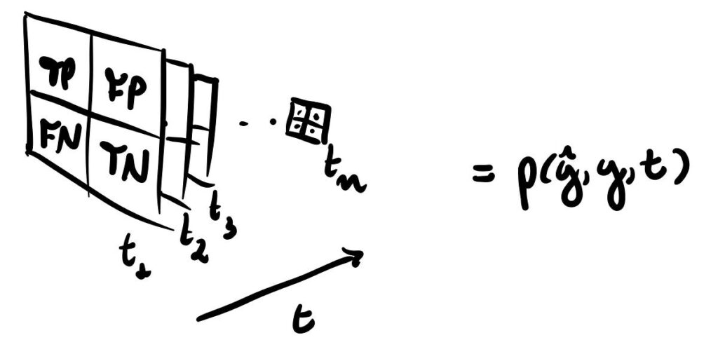
In case you are already aware of the topic, you will have observed that these are the metrics that we outline from confusion matrix of our classifier. As this matrix is outlined for every chosen choice threshold, we are able to view it as a illustration of the conditional distribution P(ŷ, y|t), the place every of those objects is a part of a category of confusion matrices that utterly describe the efficiency of our classifier.

Subsequently, the error ratios fpr and fnr are metrics that quantifies how and the way a lot the 2 conditional rating distributions intersect:

Summarizing efficiency: the ROC curve
Because the ratios are constrained by tpr + fnr = 1 and fpr + tnr = 1, this is able to imply that we have simply 2 levels of freedom to explain our efficiency.
The ROC curve is a curve parameterized by t, described by (x(t), y(t)) = (fpr(t), tpr(t)) as factors towards orthogonal axes. It will present a digestible abstract to visualise the efficiency of our classifier for all totally different threshold values, fairly than only a single one.
Your best option of t shouldn’t be typically recognized upfront however have to be decided as a part of the classifier development. — ROC Curves for Steady Knowledge (2009, Chapman and Corridor).
We’re aiming to discover the idea of treating likelihood distributions, so lets say what could be the bottom case for a totally inefficient classifier. Because the effectiveness of our predictions hinges on the discriminative nature p(s|P) and p(s|N) are, within the case the place p(s|P) = p(s|N) = p(s), we encounter a first-rate instance of this inefficiency.
If we do the train of modeling every of those conditionals as gaussians with means separated by totally different values, we are able to see how the efficiency varies clearly:

This visualization will function a invaluable support in comprehending the probabilistic interpretation of a vital classifier metric — named Space Underneath the Curve (AUC) — that we are going to delve into later.
Some properties of the ROC curve
The ROC curve might be described as a operate y = h(x) the place x and y are the false and true constructive charges respectively, that are in flip parameterized by t within the type x(t) = p(s > t|N) and and y(t) = p(s > t|P).
We are able to make the most of this to derive the next properties:
- y = h(x) is a monotone growing operate that lies above the road outlined by (0, 0) and (1, 1);
- The ROC curve is unaltered if the classification scores endure a strictly growing transformation;

This property is what makes the calibration course of for a classifier potential.
3. For a well-defined slope of ROC on the level with threshold worth t:

the place p(t|P) represents the density distribution for the cumulative distribution p(s ≤ t | P) (and identical for p(t|N)).
Binary Classification as Speculation Testing: justifying our method
When viewing the classification course of by way of a Bayesian inference lens, our goal is to infer the posterior likelihood p(P|t), which represents the chances of a degree with threshold worth t belonging to the constructive class. Subsequently, the slope by-product outlined on property 3 might be seen because the chance ratio L(t).
This ratio [L(t)] inform us how a lot possible is a worth of t of the classifier to have occurred in inhabitants P than in inhabitants N, which in flip might be interpreted as a measure of confidence in allocation to inhabitants P. — ROC Curves for Steady Knowledge (2009, Chapman and Corridor).
This is a vital reality as a result of, by establishing an equivalence relationship between the binary classification course of and speculation testing, we’ve a justification for why we classify primarily based on a threshold.
If we formulate the classification downside with the null speculation H0 that the person belongs to inhabitants N towards the choice H1 that he belongs to inhabitants P, we are able to draw the connection:

The Neyman-Pearson Lemma establishes that probably the most highly effective take a look at — which achieves the very best 1-β worth — with a significance stage α, possesses a area R encompassing all s values of S for which:

the place α is enough to find out ok by the situation p(s ∈ R|N) = α.
This means that once we rating the inhabitants in a way the place L(s) is monotonically growing, a one-to-one relationship between s and ok ensures that selecting a rule that exceeds a specific threshold is the optimum choice.
For our fictitious circumstances the place our classifier assigns a standard distribution for every class, it is direct the chance will fulfill this situation:

This isn’t all the time the case for a real-world downside, the place rating distributions usually are not essentially well-behaved on this sense. We are able to use the Kaggle dataset to know this, estimating the density of our conditionals by Kernel Density Estimation (KDE).


Because of this larger scores usually are not essentially related to a better likelihood of the person being from a constructive class.
The Space Underneath the Curve (AUC) might be probably the most broadly used worth to summarize the outcomes expressed by a ROC curve. It’s outlined because the integral of y(x) from 0 to 1, because the identify suggests. Notably, an ideal classifier’s efficiency is epitomized by the purpose (0, 1) on the orthogonal axis, denoting zero likelihood of misclassification unfavourable factors and an unambiguous assurance of appropriately classifying positives.
The method handled on determine 5 give us a touch that the probabilistic interpretation of a great match should have to do with consistency in assigning excessive rating values for constructive people and low rating for negatives ones. That is precisely the case, since one can show — as referred in [1] — that the AUC is equal to the likelihood of a constructive particular person have a rating worth (Sp) larger than a unfavourable particular person rating (Sn):

The important level to think about is that this: AUC is designed to offer a single-number estimate of your classifier’s efficiency. Nevertheless, relating to making sensible selections, a threshold t have to be chosen to go well with the precise necessities of your downside. The problem arises as a result of, as mentioned earlier, the optimum choice primarily based on a threshold happens when the chance ratio is monotonically growing, which isn’t all the time the case in apply.
Consequently, even in case you have a excessive AUC worth, very near 1, it might not be enough to find out whether or not your classifier is really able to optimum classification primarily based on a call boundary. In such circumstances, reaching a excessive AUC worth alone might not assure the effectiveness of your classifier in sensible decision-making eventualities.
This likelihood interpretation of binary classification might presents a profound understanding of the intricacies concerned within the course of. By modeling populations as distributions, we are able to make knowledgeable selections primarily based on the chance of a person belonging to a specific class. The ROC curve serves as a invaluable instrument for summarize how the selection of threshold impacts classification effectivity. Moreover, the connection between binary classification and speculation testing emphasizes the rationale why we classify by threshold values. It’s important to do not forget that whereas the Space Underneath the Curve (AUC) is a generally used efficiency metric, it might not all the time assure optimum sensible decision-making, underscoring the importance of selecting the best threshold. This probabilistic interpretation enriches our understanding of binary classification, making it a robust framework for tackling real-world issues.
Particular due to Renato Vicente, who launched me to visualizing the classifier by way of the house of confusion matrices, and inspired me to jot down this text.