A Full Information to BERT with Code | by Bradney Smith | Might, 2024

Half 4 within the “LLMs from Scratch” sequence — an entire information to understanding and constructing Massive Language Fashions. In case you are fascinated by studying extra about how these fashions work I encourage you to learn:

Bidirectional Encoder Representations from Transformers (BERT) is a Massive Language Mannequin (LLM) developed by Google AI Language which has made important developments within the area of Pure Language Processing (NLP). Many fashions lately have been impressed by or are direct enhancements to BERT, comparable to RoBERTa, ALBERT, and DistilBERT to call a couple of. The unique BERT mannequin was launched shortly after OpenAI’s Generative Pre-trained Transformer (GPT), with each constructing on the work of the Transformer structure proposed the yr prior. Whereas GPT centered on Pure Language Technology (NLG), BERT prioritised Pure Language Understanding (NLU). These two developments reshaped the panorama of NLP, cementing themselves as notable milestones within the development of machine studying.

The next article will discover the historical past of BERT, and element the panorama on the time of its creation. This may give an entire image of not solely the architectural selections made by the paper’s authors, but additionally an understanding of the way to practice and fine-tune BERT to be used in business and hobbyist functions. We are going to step by way of an in depth take a look at the structure with diagrams and write code from scratch to fine-tune BERT on a sentiment evaluation job.

1 — History and Key Features of BERT

2 — Architecture and Pre-training Objectives

3 — Fine-Tuning BERT for Sentiment Analysis

4 — Conclusion

5 — Further Reading

The BERT mannequin may be outlined by 4 predominant options:

• Encoder-only structure
• Pre-training strategy
• Mannequin fine-tuning
• Use of bidirectional context

Every of those options had been design decisions made by the paper’s authors and may be understood by contemplating the time wherein the mannequin was created. The next part will stroll by way of every of those options and present how they had been both impressed by BERT’s contemporaries (the Transformer and GPT) or supposed as an enchancment to them.

1.1 — Encoder-Solely Structure

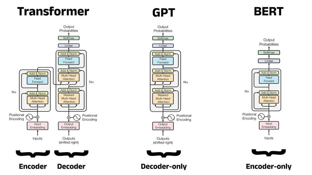
The debut of the Transformer in 2017 kickstarted a race to provide new fashions that constructed on its progressive design. OpenAI struck first in June 2018, creating GPT: a decoder-only mannequin that excelled in NLG, finally happening to energy ChatGPT in later iterations. Google responded by releasing BERT 4 months later: an encoder-only mannequin designed for NLU. Each of those architectures can produce very succesful fashions, however the duties they can carry out are barely completely different. An outline of every structure is given under.

Decoder-Solely Fashions:

• Purpose: Predict a brand new output sequence in response to an enter sequence
• Overview: The decoder block within the Transformer is chargeable for producing an output sequence primarily based on the enter supplied to the encoder. Decoder-only fashions are constructed by omitting the encoder block solely and stacking a number of decoders collectively in a single mannequin. These fashions settle for prompts as inputs and generate responses by predicting the following most possible phrase (or extra particularly, token) one after the other in a job generally known as Subsequent Token Prediction (NTP). In consequence, decoder-only fashions excel in NLG duties comparable to: conversational chatbots, machine translation, and code technology. These sorts of fashions are doubtless essentially the most acquainted to most of the people because of the widespread use of ChatGPT which is powered by decoder-only fashions (GPT-3.5 and GPT-4).

Encoder-Solely Fashions:

• Purpose: Make predictions about phrases inside an enter sequence
• Overview: The encoder block within the Transformer is chargeable for accepting an enter sequence, and creating wealthy, numeric vector representations for every phrase (or extra particularly, every token). Encoder-only fashions omit the decoder and stack a number of Transformer encoders to provide a single mannequin. These fashions don’t settle for prompts as such, however fairly an enter sequence for a prediction to be made upon (e.g. predicting a lacking phrase throughout the sequence). Encoder-only fashions lack the decoder used to generate new phrases, and so should not used for chatbot functions in the best way that GPT is used. As a substitute, encoder-only fashions are most frequently used for NLU duties comparable to: Named Entity Recognition (NER) and sentiment evaluation. The wealthy vector representations created by the encoder blocks are what give BERT a deep understanding of the enter textual content. The BERT authors argued that this architectural alternative would enhance BERT’s efficiency in comparison with GPT, particularly writing that decoder-only architectures are:

“sub-optimal for sentence-level duties, and could possibly be very dangerous when making use of finetuning primarily based approaches to token-level duties comparable to query answering” [1]

Notice: It’s technically doable to generate textual content with BERT, however as we are going to see, this isn’t what the structure was supposed for, and the outcomes don’t rival decoder-only fashions in any approach.

Structure Diagrams for the Transformer, GPT, and BERT:

Under is an structure diagram for the three fashions we now have mentioned to date. This has been created by adapting the structure diagram from the unique Transformer paper “Consideration is All You Want” [2]. The variety of encoder or decoder blocks for the mannequin is denoted by N. Within the authentic Transformer, N is the same as 6 for the encoder and 6 for the decoder, since these are each made up of six encoder and decoder blocks stacked collectively respectively.

1.2 — Pre-training Strategy

GPT influenced the event of BERT in a number of methods. Not solely was the mannequin the primary decoder-only Transformer by-product, however GPT additionally popularised mannequin pre-training. Pre-training entails coaching a single giant mannequin to amass a broad understanding of language (encompassing features comparable to phrase utilization and grammatical patterns) with a view to produce a task-agnostic foundational mannequin. Within the diagrams above, the foundational mannequin is made up of the parts under the linear layer (proven in purple). As soon as skilled, copies of this foundational mannequin may be fine-tuned to deal with particular duties. Tremendous-tuning entails coaching solely the linear layer: a small feedforward neural community, typically known as a classification head or only a head. The weights and biases within the the rest of the mannequin (that’s, the foundational portion) remained unchanged, or frozen.

Analogy:

To assemble a quick analogy, take into account a sentiment evaluation job. Right here, the aim is to categorise textual content as both constructive or detrimental primarily based on the sentiment portrayed. For instance, in some film critiques, textual content comparable to I liked this film can be labeled as constructive and textual content comparable to I hated this film can be labeled as detrimental. Within the conventional strategy to language modelling, you’ll doubtless practice a brand new structure from scratch particularly for this one job. You can consider this as educating somebody the English language from scratch by displaying them film critiques till finally they can classify the sentiment discovered inside them. This in fact, can be sluggish, costly, and require many coaching examples. Furthermore, the ensuing classifier would nonetheless solely be proficient on this one job. Within the pre-training strategy, you’re taking a generic mannequin and fine-tune it for sentiment evaluation. You possibly can consider this as taking somebody who’s already fluent in English and easily displaying them a small variety of film critiques to familiarise them with the present job. Hopefully, it’s intuitive that the second strategy is way more environment friendly.

Earlier Makes an attempt at Pre-training:

The idea of pre-training was not invented by OpenAI, and had been explored by different researchers within the years prior. One notable instance is the ELMo mannequin (Embeddings from Language Fashions), developed by researchers on the Allen Institute [3]. Regardless of these earlier makes an attempt, no different researchers had been capable of reveal the effectiveness of pre-training as convincingly as OpenAI of their seminal paper. In their very own phrases, the crew discovered that their

“task-agnostic mannequin outperforms discriminatively skilled fashions that use architectures particularly crafted for every job, considerably bettering upon the cutting-edge” [4].

This revelation firmly established the pre-training paradigm because the dominant strategy to language modelling transferring ahead. Consistent with this pattern, the BERT authors additionally totally adopted the pre-trained strategy.

1.3 — Mannequin Tremendous-tuning

Advantages of Tremendous-tuning:

Tremendous-tuning has turn out to be commonplace at the moment, making it simple to miss how latest it was that this strategy rose to prominence. Previous to 2018, it was typical for a brand new mannequin structure to be launched for every distinct NLP job. Transitioning to pre-training not solely drastically decreased the coaching time and compute value wanted to develop a mannequin, but additionally lowered the amount of coaching knowledge required. Fairly than fully redesigning and retraining a language mannequin from scratch, a generic mannequin like GPT could possibly be fine-tuned with a small quantity of task-specific knowledge in a fraction of the time. Relying on the duty, the classification head may be modified to include a special variety of output neurons. That is helpful for classification duties comparable to sentiment evaluation. For instance, if the specified output of a BERT mannequin is to foretell whether or not a evaluate is constructive or detrimental, the pinnacle may be modified to characteristic two output neurons. The activation of every signifies the likelihood of the evaluate being constructive or detrimental respectively. For a multi-class classification job with 10 courses, the pinnacle may be modified to have 10 neurons within the output layer, and so forth. This makes BERT extra versatile, permitting the foundational mannequin for use for varied downstream duties.

Tremendous-tuning in BERT:

BERT adopted within the footsteps of GPT and in addition took this pre-training/fine-tuning strategy. Google launched two variations of BERT: Base and Massive, providing customers flexibility in mannequin dimension primarily based on {hardware} constraints. Each variants took round 4 days to pre-train on many TPUs (tensor processing items), with BERT Base skilled on 16 TPUs and BERT Massive skilled on 64 TPUs. For many researchers, hobbyists, and business practitioners, this stage of coaching wouldn’t be possible. Therefore, the concept of spending just a few hours fine-tuning a foundational mannequin on a specific job stays a way more interesting various. The unique BERT structure has undergone 1000’s of fine-tuning iterations throughout varied duties and datasets, lots of that are publicly accessible for obtain on platforms like Hugging Face [5].

1.4 — Use of Bidirectional Context

As a language mannequin, BERT predicts the likelihood of observing sure phrases on condition that prior phrases have been noticed. This elementary side is shared by all language fashions, no matter their structure and supposed job. Nonetheless, it’s the utilisation of those possibilities that offers the mannequin its task-specific behaviour. For instance, GPT is skilled to foretell the following most possible phrase in a sequence. That’s, the mannequin predicts the following phrase, on condition that the earlier phrases have been noticed. Different fashions is likely to be skilled on sentiment evaluation, predicting the sentiment of an enter sequence utilizing a textual label comparable to constructive or detrimental, and so forth. Making any significant predictions about textual content requires the encircling context to be understood, particularly in NLU duties. BERT ensures good understanding by way of certainly one of its key properties: bidirectionality.

Bidirectionality is probably BERT’s most important characteristic and is pivotal to its excessive efficiency in NLU duties, in addition to being the driving purpose behind the mannequin’s encoder-only structure. Whereas the self-attention mechanism of Transformer encoders calculates bidirectional context, the identical can’t be mentioned for decoders which produce unidirectional context. The BERT authors argued that this lack of bidirectionality in GPT prevents it from attaining the identical depth of language illustration as BERT.

Defining Bidirectionality:

However what precisely does “bidirectional” context imply? Right here, bidirectional denotes that every phrase within the enter sequence can achieve context from each previous and succeeding phrases (known as the left context and proper context respectively). In technical phrases, we are saying that the eye mechanism can attend to the previous and subsequent tokens for every phrase. To interrupt this down, recall that BERT solely makes predictions about phrases inside an enter sequence, and doesn’t generate new sequences like GPT. Due to this fact, when BERT predicts a phrase throughout the enter sequence, it might probably incorporate contextual clues from all the encircling phrases. This provides context in each instructions, serving to BERT to make extra knowledgeable predictions.

Distinction this with decoder-only fashions like GPT, the place the target is to foretell new phrases one after the other to generate an output sequence. Every predicted phrase can solely leverage the context supplied by previous phrases (left context) as the next phrases (proper context) haven’t but been generated. Due to this fact, these fashions are known as unidirectional.

Picture Breakdown:

The picture above reveals an instance of a typical BERT job utilizing bidirectional context, and a typical GPT job utilizing unidirectional context. For BERT, the duty right here is to foretell the masked phrase indicated by [MASK]. Since this phrase has phrases to each the left and proper, the phrases from both aspect can be utilized to supply context. In the event you, as a human, learn this sentence with solely the left or proper context, you’ll most likely wrestle to foretell the masked phrase your self. Nonetheless, with bidirectional context it turns into more likely to guess that the masked phrase is fishing.

For GPT, the aim is to carry out the traditional NTP job. On this case, the target is to generate a brand new sequence primarily based on the context supplied by the enter sequence and the phrases already generated within the output. Provided that the enter sequence instructs the mannequin to write down a poem and the phrases generated to date are Upon a, you would possibly predict that the following phrase is river adopted by financial institution. With many potential candidate phrases, GPT (as a language mannequin) calculates the chance of every phrase in its vocabulary showing subsequent and selects one of the vital possible phrases primarily based on its coaching knowledge.

1.5 — Limitations of BERT

As a bidirectional mannequin, BERT suffers from two main drawbacks:

Elevated Coaching Time:

Bidirectionality in Transformer-based fashions was proposed as a direct enchancment over the left-to-right context fashions prevalent on the time. The concept was that GPT might solely achieve contextual details about enter sequences in a unidirectional method and subsequently lacked an entire grasp of the causal hyperlinks between phrases. Bidirectional fashions, nevertheless, supply a broader understanding of the causal connections between phrases and so can doubtlessly see higher outcomes on NLU duties. Although bidirectional fashions had been explored previously, their success was restricted, as seen with bidirectional RNNs within the late Nineteen Nineties [6]. Usually, these fashions demand extra computational sources for coaching, so for a similar computational energy you would practice a bigger unidirectional mannequin.

Poor Efficiency in Language Technology:

BERT was particularly designed to unravel NLU duties, opting to commerce decoders and the flexibility to generate new sequences for encoders and the flexibility to develop wealthy understandings of enter sequences. In consequence, BERT is greatest suited to a subset of NLP duties like NER, sentiment evaluation and so forth. Notably, BERT doesn’t settle for prompts however fairly processes sequences to formulate predictions about. Whereas BERT can technically produce new output sequences, it is very important recognise the design variations between LLMs as we’d consider them within the post-ChatGPT period, and the fact of BERT’s design.

2.1 — Overview of BERT’s Pre-training Targets

Coaching a bidirectional mannequin requires duties that enable each the left and proper context for use in making predictions. Due to this fact, the authors fastidiously constructed two pre-training targets to construct up BERT’s understanding of language. These had been: the Masked Language Mannequin job (MLM), and the Subsequent Sentence Prediction job (NSP). The coaching knowledge for every was constructed from a scrape of all of the English Wikipedia articles out there on the time (2,500 million phrases), and an extra 11,038 books from the BookCorpus dataset (800 million phrases) [7]. The uncooked knowledge was first preprocessed in accordance with the particular duties nevertheless, as described under.

2.2 — Masked Language Modelling (MLM)

Overview of MLM:

The Masked Language Modelling job was created to immediately tackle the necessity for coaching a bidirectional mannequin. To take action, the mannequin should be skilled to make use of each the left context and proper context of an enter sequence to make a prediction. That is achieved by randomly masking 15% of the phrases within the coaching knowledge, and coaching BERT to foretell the lacking phrase. Within the enter sequence, the masked phrase is changed with the [MASK] token. For instance, take into account that the sentence A person was fishing on the river exists within the uncooked coaching knowledge discovered within the ebook corpus. When changing the uncooked textual content into coaching knowledge for the MLM job, the phrase fishing is likely to be randomly masked and changed with the [MASK] token, giving the coaching enter A person was [MASK] on the river with goal fishing. Due to this fact, the aim of BERT is to foretell the only lacking phrase fishing, and never regenerate the enter sequence with the lacking phrase stuffed in. The masking course of may be repeated for all of the doable enter sequences (e.g. sentences) when build up the coaching knowledge for the MLM job. This job had existed beforehand in linguistics literature, and is known as the Cloze job [8]. Nonetheless, in machine studying contexts, it’s generally known as MLM because of the reputation of BERT.

Mitigating Mismatches Between Pre-training and Tremendous-tuning:

The authors famous nevertheless, that for the reason that [MASK] token will solely ever seem within the coaching knowledge and never in stay knowledge (at inference time), there can be a mismatch between pre-training and fine-tuning. To mitigate this, not all masked phrases are changed with the [MASK] token. As a substitute, the authors state that:

The coaching knowledge generator chooses 15% of the token positions at random for prediction. If the i-th token is chosen, we change the i-th token with (1) the [MASK] token 80% of the time (2) a random token 10% of the time (3) the unchanged i-th token 10% of the time.

Calculating the Error Between the Predicted Phrase and the Goal Phrase:

BERT will soak up an enter sequence of a most of 512 tokens for each BERT Base and BERT Massive. If fewer than the utmost variety of tokens are discovered within the sequence, then padding will likely be added utilizing [PAD] tokens to achieve the utmost depend of 512. The variety of output tokens may even be precisely equal to the variety of enter tokens. If a masked token exists at place i within the enter sequence, BERT’s prediction will lie at place i within the output sequence. All different tokens will likely be ignored for the needs of coaching, and so updates to the fashions weights and biases will likely be calculated primarily based on the error between the anticipated token at place i, and the goal token. The error is calculated utilizing a loss perform, which is often the Cross Entropy Loss (Damaging Log Chance) perform, as we are going to see later.

2.3 — Subsequent Sentence Prediction (NSP)

Overview:

The second of BERT’s pre-training duties is Subsequent Sentence Prediction, wherein the aim is to categorise if one phase (usually a sentence) logically follows on from one other. The selection of NSP as a pre-training job was made particularly to enhance MLM and improve BERT’s NLU capabilities, with the authors stating:

Many necessary downstream duties comparable to Query Answering (QA) and Pure Language Inference (NLI) are primarily based on understanding the connection between two sentences, which isn’t immediately captured by language modeling.

By pre-training for NSP, BERT is ready to develop an understanding of circulation between sentences in prose textual content — a capability that’s helpful for a variety of NLU issues, comparable to:

• sentence pairs in paraphrasing
• hypothesis-premise pairs in entailment
• question-passage pairs in query answering

Implementing NSP in BERT:

The enter for NSP consists of the primary and second segments (denoted A and B) separated by a [SEP] token with a second [SEP] token on the finish. BERT really expects a minimum of one [SEP] token per enter sequence to indicate the tip of the sequence, no matter whether or not NSP is being carried out or not. For that reason, the WordPiece tokenizer will append certainly one of these tokens to the tip of inputs for the MLM job in addition to another non-NSP job that don’t characteristic one. NSP types a classification downside, the place the output corresponds to IsNext when phase A logically follows phase B, and NotNext when it doesn’t. Coaching knowledge may be simply generated from any monolingual corpus by deciding on sentences with their subsequent sentence 50% of the time, and a random sentence for the remaining 50% of sentences.

2.4 — Enter Embeddings in BERT

The enter embedding course of for BERT is made up of three phases: positional encoding, phase embedding, and token embedding (as proven within the diagram under).

Positional Encoding:

Simply as with the Transformer mannequin, positional info is injected into the embedding for every token. Not like the Transformer nevertheless, the positional encodings in BERT are fastened and never generated by a perform. Which means that BERT is restricted to 512 tokens in its enter sequence for each BERT Base and BERT Massive.

Section Embedding:

Vectors encoding the phase that every token belongs to are additionally added. For the MLM pre-training job or another non-NSP job (which characteristic just one [SEP]) token, all tokens within the enter are thought-about to belong to phase A. For NSP duties, all tokens after the second [SEP] are denoted as phase B.

Token Embedding:

As with the unique Transformer, the discovered embedding for every token is then added to its positional and phase vectors to create the ultimate embedding that will likely be handed to the self-attention mechanisms in BERT so as to add contextual info.

2.5 — The Particular Tokens

Within the picture above, you will have famous that the enter sequence has been prepended with a [CLS] (classification) token. This token is added to encapsulate a abstract of the semantic that means of all the enter sequence, and helps BERT to carry out classification duties. For instance, within the sentiment evaluation job, the [CLS] token within the last layer may be analysed to extract a prediction for whether or not the sentiment of the enter sequence is constructive or detrimental. [CLS] and [PAD] and so on are examples of BERT’s particular tokens. It’s necessary to notice right here that it is a BERT-specific characteristic, and so you shouldn’t anticipate to see these particular tokens in fashions comparable to GPT. In whole, BERT has 5 particular tokens. A abstract is supplied under:

• [PAD] (token ID: 0) — a padding token used to convey the overall variety of tokens in an enter sequence as much as 512.
• [UNK] (token ID: 100) — an unknown token, used to symbolize a token that isn’t in BERT’s vocabulary.
• [CLS] (token ID: 101) — a classification token, one is predicted firstly of each sequence, whether or not it’s used or not. This token encapsulates the category info for classification duties, and may be considered an mixture sequence illustration.
• [SEP] (token ID: 102) — a separator token used to differentiate between two segments in a single enter sequence (for instance, in Subsequent Sentence Prediction). At the least one [SEP] token is predicted per enter sequence, with a most of two.
• [MASK] (token ID: 103) — a masks token used to coach BERT on the Masked Language Modelling job, or to carry out inference on a masked sequence.

2.4 — Structure Comparability for BERT Base and BERT Massive

BERT Base and BERT Massive are very comparable from an structure point-of-view, as you would possibly anticipate. They each use the WordPiece tokenizer (and therefore anticipate the identical particular tokens described earlier), and each have a most sequence size of 512 tokens. The vocabulary dimension for BERT is 30,522, with roughly 1,000 of these tokens left as “unused”. The unused tokens are deliberately left clean to permit customers so as to add customized tokens with out having to retrain all the tokenizer. That is helpful when working with domain-specific vocabulary, comparable to medical and authorized terminology. Each BERT Base and BERT Massive have the next variety of embedding dimensions (d_model) in comparison with the unique Transformer. This corresponds to the dimensions of the discovered vector representations for every token within the mannequin’s vocabulary. For BERT Base d_model = 768, and for BERT Massive d_model = 1024 (double the unique Transformer at 512).

The 2 fashions primarily differ in 4 classes:

• Variety of encoder blocks, N: the variety of encoder blocks stacked on prime of one another.
• Variety of consideration heads per encoder block: the eye heads calculate the contextual vector embeddings for the enter sequence. Since BERT makes use of multi-head consideration, this worth refers back to the variety of heads per encoder layer.
• Measurement of hidden layer in feedforward community: the linear layer consists of a hidden layer with a set variety of neurons (e.g. 3072 for BERT Base) which feed into an output layer that may be of assorted sizes. The scale of the output layer depends upon the duty. As an illustration, a binary classification downside would require simply two output neurons, a multi-class classification downside with ten courses would require ten neurons, and so forth.
• Complete parameters: the overall variety of weights and biases within the mannequin. On the time, a mannequin with a whole lot of hundreds of thousands was very giant. Nonetheless, by at the moment’s requirements, these values are comparatively small.

A comparability between BERT Base and BERT Massive for every of those classes is proven within the picture under.

This part covers a sensible instance of fine-tuning BERT in Python. The code takes the type of a task-agnostic fine-tuning pipeline, carried out in a Python class. We are going to then instantiate an object of this class and use it to fine-tune a BERT mannequin on the sentiment evaluation job. The category may be reused to fine-tune BERT on different duties, comparable to Query Answering, Named Entity Recognition, and extra. Sections 3.1 to three.5 stroll by way of the fine-tuning course of, and Part 3.6 reveals the complete pipeline in its entirety.

3.1 — Load and Preprocess a Tremendous-Tuning Dataset

Step one in fine-tuning is to pick out a dataset that’s appropriate for the particular job. On this instance, we are going to use a sentiment evaluation dataset supplied by Stanford College. This dataset incorporates 50,000 on-line film critiques from the Web Film Database (IMDb), with every evaluate labelled as both constructive or detrimental. You possibly can obtain the dataset immediately from the Stanford University website, or you’ll be able to create a pocket book on Kaggle and examine your work with others.

import pandas as pd
df = pd.read_csv('IMDB Dataset.csv')
df.head()

Not like earlier NLP fashions, Transformer-based fashions comparable to BERT require minimal preprocessing. Steps comparable to eradicating cease phrases and punctuation can show counterproductive in some circumstances, since these components present BERT with helpful context for understanding the enter sentences. However, it’s nonetheless necessary to examine the textual content to verify for any formatting points or undesirable characters. Total, the IMDb dataset is pretty clear. Nonetheless, there seem like some artefacts of the scraping course of leftover, comparable to HTML break tags (<br />) and pointless whitespace, which ought to be eliminated.

# Take away the break tags (<br />)
df['review_cleaned'] = df['review'].apply(lambda x: x.change('<br />', ''))
# Take away pointless whitespace
df['review_cleaned'] = df['review_cleaned'].change('s+', ' ', regex=True)
# Examine 72 characters of the second evaluate earlier than and after cleansing
print('Earlier than cleansing:')
print(df.iloc[1]['review'][0:72])
print('nAfter cleansing:')
print(df.iloc[1]['review_cleaned'][0:72])

Earlier than cleansing:
A beautiful little manufacturing. <br /><br />The filming approach could be very
After cleansing:
A beautiful little manufacturing. The filming approach could be very unassuming-

Encode the Sentiment:

The ultimate step of the preprocessing is to encode the sentiment of every evaluate as both 0 for detrimental or 1 for constructive. These labels will likely be used to coach the classification head later within the fine-tuning course of.

df['sentiment_encoded'] = df['sentiment'].
apply(lambda x: 0 if x == 'detrimental' else 1)
df.head()

3.2 — Tokenize the Tremendous-Tuning Knowledge

As soon as preprocessed, the fine-tuning knowledge can endure tokenization. This course of: splits the evaluate textual content into particular person tokens, provides the [CLS] and [SEP] particular tokens, and handles padding. It’s necessary to pick out the suitable tokenizer for the mannequin, as completely different language fashions require completely different tokenization steps (e.g. GPT doesn’t anticipate [CLS] and [SEP] tokens). We are going to use the BertTokenizer class from the Hugging Face transformers library, which is designed for use with BERT-based fashions. For a extra in-depth dialogue of how tokenization works, see Part 1 of this series.

Tokenizer courses within the transformers library present a easy technique to create pre-trained tokenizer fashions with the from_pretrained technique. To make use of this characteristic: import and instantiate a tokenizer class, name the from_pretrained technique, and move in a string with the identify of a tokenizer mannequin hosted on the Hugging Face mannequin repository. Alternatively, you’ll be able to move within the path to a listing containing the vocabulary recordsdata required by the tokenizer [9]. For our instance, we are going to use a pre-trained tokenizer from the mannequin repository. There are 4 predominant choices when working with BERT, every of which use the vocabulary from Google’s pre-trained tokenizers. These are:

• bert-base-uncased — the vocabulary for the smaller model of BERT, which is NOT case delicate (e.g. the tokens Cat and cat will likely be handled the identical)
• bert-base-cased — the vocabulary for the smaller model of BERT, which IS case delicate (e.g. the tokens Cat and cat is not going to be handled the identical)
• bert-large-uncased — the vocabulary for the bigger model of BERT, which is NOT case delicate (e.g. the tokens Cat and cat will likely be handled the identical)
• bert-large-cased — the vocabulary for the bigger model of BERT, which IS case delicate (e.g. the tokens Cat and cat is not going to be handled the identical)

Each BERT Base and BERT Massive use the identical vocabulary, and so there may be really no distinction between bert-base-uncased and bert-large-uncased, neither is there a distinction between bert-base-cased and bert-large-cased. This is probably not the identical for different fashions, so it’s best to make use of the identical tokenizer and mannequin dimension in case you are uncertain.

When to Use cased vs uncased:

The choice between utilizing cased and uncased depends upon the character of your dataset. The IMDb dataset incorporates textual content written by web customers who could also be inconsistent with their use of capitalisation. For instance, some customers might omit capitalisation the place it’s anticipated, or use capitalisation for dramatic impact (to indicate pleasure, frustration, and so on). For that reason, we are going to select to disregard case and use the bert-base-uncased tokenizer mannequin.

Different conditions might even see a efficiency profit by accounting for case. An instance right here could also be in a Named Entity Recognition job, the place the aim is to establish entities comparable to individuals, organisations, areas, and so on in some enter textual content. On this case, the presence of higher case letters may be extraordinarily useful in figuring out if a phrase is somebody’s identify or a spot, and so on this scenario it could be extra acceptable to decide on bert-base-cased.

from transformers import BertTokenizer
tokenizer = BertTokenizer.from_pretrained('bert-base-uncased')
print(tokenizer)

BertTokenizer(
name_or_path='bert-base-uncased',
vocab_size=30522,
model_max_length=512,
is_fast=False,
padding_side='proper',
truncation_side='proper',
special_tokens={
'unk_token': '[UNK]',
'sep_token': '[SEP]',
'pad_token': '[PAD]',
'cls_token': '[CLS]',
'mask_token': '[MASK]'},
clean_up_tokenization_spaces=True),
added_tokens_decoder={
0: AddedToken(
"[PAD]",
rstrip=False,
lstrip=False,
single_word=False,
normalized=False,  
particular=True),
100: AddedToken(
"[UNK]",
rstrip=False,
lstrip=False,
single_word=False,
normalized=False,
particular=True),
101: AddedToken(
"[CLS]",
rstrip=False,
lstrip=False,
single_word=False,
normalized=False,
particular=True),
102: AddedToken(
"[SEP]",
rstrip=False,
lstrip=False,
single_word=False,
normalized=False,
particular=True),
103: AddedToken(
"[MASK]",
rstrip=False,
lstrip=False,
single_word=False,
normalized=False,
particular=True),
}

Encoding Course of: Changing Textual content to Tokens to Token IDs

Subsequent, the tokenizer can be utilized to encode the cleaned fine-tuning knowledge. This course of will convert every evaluate right into a tensor of token IDs. For instance, the evaluate I favored this film will likely be encoded by the next steps:

1. Convert the evaluate to decrease case (since we’re utilizing bert-base-uncased)

2. Break the evaluate down into particular person tokens in accordance with the bert-base-uncased vocabulary: ['i', 'liked', 'this', 'movie']

2. Add the particular tokens anticipated by BERT: ['[CLS]', 'i', 'favored', 'this', 'film', '[SEP]']

3. Convert the tokens to their token IDs, additionally in accordance with the bert-base-uncased vocabulary (e.g. [CLS] -> 101, i -> 1045, and so on)

The encode technique of the BertTokenizer class encodes textual content utilizing the above course of, and might return the tensor of token IDs as PyTorch tensors, Tensorflow tensors, or NumPy arrays. The info sort for the return tensor may be specified utilizing the return_tensors argument, which takes the values: pt, tf, and np respectively.

Notice: Token IDs are sometimes known as enter IDs in Hugging Face, so you might even see these phrases used interchangeably.

# Encode a pattern enter sentence
sample_sentence = 'I favored this film'
token_ids = tokenizer.encode(sample_sentence, return_tensors='np')[0]
print(f'Token IDs: {token_ids}')
# Convert the token IDs again to tokens to disclose the particular tokens added
tokens = tokenizer.convert_ids_to_tokens(token_ids)
print(f'Tokens   : {tokens}')

Token IDs: [ 101 1045 4669 2023 3185  102]
Tokens   : ['[CLS]', 'i', 'favored', 'this', 'film', '[SEP]']

Truncation and Padding:

Each BERT Base and BERT Massive are designed to deal with enter sequences of precisely 512 tokens. However what do you do when your enter sequence doesn’t match this restrict? The reply is truncation and padding! Truncation reduces the variety of tokens by merely eradicating any tokens past a sure size. Within the encode technique, you’ll be able to set truncation to True and specify a max_length argument to implement a size restrict on all encoded sequences. A number of of the entries on this dataset exceed the 512 token restrict, and so the max_length parameter right here has been set to 512 to extract essentially the most quantity of textual content doable from all critiques. If no evaluate exceeds 512 tokens, the max_length parameter may be left unset and it’ll default to the mannequin’s most size. Alternatively, you’ll be able to nonetheless implement a most size which is lower than 512 to scale back coaching time throughout fine-tuning, albeit on the expense of mannequin efficiency. For critiques shorter than 512 tokens (which is almost all right here), padding tokens are added to increase the encoded evaluate to 512 tokens. This may be achieved by setting the padding parameter to max_length. Confer with the Hugging Face documentation for extra particulars on the encode technique [10].

evaluate = df['review_cleaned'].iloc[0]
token_ids = tokenizer.encode(
evaluate,
max_length = 512,
padding = 'max_length',
truncation = True,
return_tensors = 'pt')
print(token_ids)

tensor([[  101,  2028,  1997,  1996,  2060, 15814,  2038,  3855,  2008,  2044,
3666,  2074,  1015, 11472,  2792,  2017,  1005,  2222,  2022, 13322,
...
0,     0,     0,     0,     0,     0,     0,     0,     0,     0,
0,     0,     0,     0,     0,     0,     0,     0,     0,     0,
0,     0]])

Utilizing the Consideration Masks with encode_plus:

The instance above reveals the encoding for the primary evaluate within the dataset, which incorporates 119 padding tokens. If utilized in its present state for fine-tuning, BERT might attend to the padding tokens, doubtlessly resulting in a drop in efficiency. To deal with this, we are able to apply an consideration masks that may instruct BERT to disregard sure tokens within the enter (on this case the padding tokens). We will generate this consideration masks by modifying the code above to make use of the encode_plus technique, fairly than the usual encode technique. The encode_plus technique returns a dictionary (known as a Batch Encoder in Hugging Face), which incorporates the keys:

• input_ids — the identical token IDs returned by the usual encode technique
• token_type_ids — the phase IDs used to differentiate between sentence A (id = 0) and sentence B (id = 1) in sentence pair duties comparable to Subsequent Sentence Prediction
• attention_mask — a listing of 0s and 1s the place 0 signifies {that a} token ought to be ignored through the consideration course of and 1 signifies a token shouldn’t be ignored

evaluate = df['review_cleaned'].iloc[0]
batch_encoder = tokenizer.encode_plus(
evaluate,
max_length = 512,
padding = 'max_length',
truncation = True,
return_tensors = 'pt')
print('Batch encoder keys:')
print(batch_encoder.keys())
print('nAttention masks:')
print(batch_encoder['attention_mask'])

Batch encoder keys:
dict_keys(['input_ids', 'token_type_ids', 'attention_mask'])
Consideration masks:
tensor([[1, 1, 1, 1, 1, 1, 1, 1, 1, 1, 1, 1, 1, 1, 1, 1, 1, 1, 1, 1, 1, 1, 1,
1, 1, 1, 1, 1, 1, 1, 1, 1, 1, 1, 1, 1, 1, 1, 1, 1, 1, 1, 1, 1, 1, 1,
...
0, 0, 0, 0, 0, 0, 0, 0, 0, 0, 0, 0, 0, 0, 0, 0, 0, 0, 0, 0, 0, 0, 0,
0, 0, 0, 0, 0, 0, 0, 0, 0, 0, 0, 0, 0, 0, 0, 0, 0, 0, 0, 0, 0, 0, 0, 
0, 0, 0, 0, 0, 0, 0, 0]])

Encode All Evaluations:

The final step for the tokenization stage is to encode all of the critiques within the dataset and retailer the token IDs and corresponding consideration masks as tensors.

import torch
token_ids = []
attention_masks = []
# Encode every evaluate
for evaluate in df['review_cleaned']:
batch_encoder = tokenizer.encode_plus(
evaluate,
max_length = 512,
padding = 'max_length',
truncation = True,
return_tensors = 'pt')
token_ids.append(batch_encoder['input_ids'])
attention_masks.append(batch_encoder['attention_mask'])
# Convert token IDs and a spotlight masks lists to PyTorch tensors
token_ids = torch.cat(token_ids, dim=0)
attention_masks = torch.cat(attention_masks, dim=0)

3.3 — Create the Practice and Validation DataLoaders

Now that every evaluate has been encoded, we are able to cut up our knowledge right into a coaching set and a validation set. The validation set will likely be used to judge the effectiveness of the fine-tuning course of because it occurs, permitting us to observe the efficiency all through the method. We anticipate to see a lower in loss (and consequently a rise in mannequin accuracy) because the mannequin undergoes additional fine-tuning throughout epochs. An epoch refers to at least one full move of the practice knowledge. The BERT authors suggest 2–4 epochs for fine-tuning [1], that means that the classification head will see each evaluate 2–4 instances.

To partition the info, we are able to use the train_test_split perform from SciKit-Study’s model_selection package deal. This perform requires the dataset we intend to separate, the proportion of things to be allotted to the take a look at set (or validation set in our case), and an non-compulsory argument for whether or not the info ought to be randomly shuffled. For reproducibility, we are going to set the shuffle parameter to False. For the test_size, we are going to select a small worth of 0.1 (equal to 10%). You will need to strike a stability between utilizing sufficient knowledge to validate the mannequin and get an correct image of how it’s performing, and retaining sufficient knowledge for coaching the mannequin and bettering its efficiency. Due to this fact, smaller values comparable to 0.1 are sometimes most popular. After the token IDs, consideration masks, and labels have been cut up, we are able to group the coaching and validation tensors collectively in PyTorch TensorDatasets. We will then create a PyTorch DataLoader class for coaching and validation by dividing these TensorDatasets into batches. The BERT paper recommends batch sizes of 16 or 32 (that’s, presenting the mannequin with 16 critiques and corresponding sentiment labels earlier than recalculating the weights and biases within the classification head). Utilizing DataLoaders will enable us to effectively load the info into the mannequin through the fine-tuning course of by exploiting a number of CPU cores for parallelisation [11].

from sklearn.model_selection import train_test_split
from torch.utils.knowledge import TensorDataset, DataLoader
val_size = 0.1
# Cut up the token IDs
train_ids, val_ids = train_test_split(
token_ids,
test_size=val_size,
shuffle=False)
# Cut up the eye masks
train_masks, val_masks = train_test_split(
attention_masks,
test_size=val_size,
shuffle=False)
# Cut up the labels
labels = torch.tensor(df['sentiment_encoded'].values)
train_labels, val_labels = train_test_split(
labels,
test_size=val_size,
shuffle=False)
# Create the DataLoaders
train_data = TensorDataset(train_ids, train_masks, train_labels)
train_dataloader = DataLoader(train_data, shuffle=True, batch_size=16)
val_data = TensorDataset(val_ids, val_masks, val_labels)
val_dataloader = DataLoader(val_data, batch_size=16)

3.4 — Instantiate a BERT Mannequin

The subsequent step is to load in a pre-trained BERT mannequin for us to fine-tune. We will import a mannequin from the Hugging Face mannequin repository equally to how we did with the tokenizer. Hugging Face has many variations of BERT with classification heads already connected, which makes this course of very handy. Some examples of fashions with pre-configured classification heads embrace:

• BertForMaskedLM
• BertForNextSentencePrediction
• BertForSequenceClassification
• BertForMultipleChoice
• BertForTokenClassification
• BertForQuestionAnswering

After all, it’s doable to import a headless BERT mannequin and create your individual classification head from scratch in PyTorch or Tensorflow. Nonetheless in our case, we are able to merely import the BertForSequenceClassification mannequin since this already incorporates the linear layer we want. This linear layer is initialised with random weights and biases, which will likely be skilled through the fine-tuning course of. Since BERT Base makes use of 768 embedding dimensions, the hidden layer incorporates 768 neurons that are linked to the ultimate encoder block of the mannequin. The variety of output neurons is decided by the num_labels argument, and corresponds to the variety of distinctive sentiment labels. The IMDb dataset options solely constructive and detrimental, and so the num_labels argument is about to 2. For extra complicated sentiment analyses, maybe together with labels comparable to impartial or blended, we are able to merely enhance/lower the num_labels worth.

Notice: In case you are fascinated by seeing how the pre-configured fashions are written within the supply code, the modelling_bert.py file on the Hugging Face transformers repository reveals the method of loading in a headless BERT mannequin and including the linear layer [12]. The linear layer is added within the __init__ technique of every class.

from transformers import BertForSequenceClassification
mannequin = BertForSequenceClassification.from_pretrained(
'bert-base-uncased',
num_labels=2)

3.5 — Instantiate an Optimizer, Loss Perform, and Scheduler

Optimizer:

After the classification head encounters a batch of coaching knowledge, it updates the weights and biases within the linear layer to enhance the mannequin’s efficiency on these inputs. Throughout many batches and a number of epochs, the intention is for these weights and biases to converge in direction of optimum values. An optimizer is required to calculate the adjustments wanted to every weight and bias, and may be imported from PyTorch’s `optim` package deal. Hugging Face use the AdamW optimizer of their examples, and so that is the optimizer we are going to use right here [13].

Loss Perform:

The optimizer works by figuring out how adjustments to the weights and biases within the classification head will have an effect on the loss in opposition to a scoring perform known as the loss perform. Loss capabilities may be simply imported from PyTorch’s nn package deal, as proven under. Language fashions usually use the cross entropy loss perform (additionally known as the detrimental log chance perform), and so that is the loss perform we are going to use right here.

Scheduler:

A parameter known as the studying price is used to find out the dimensions of the adjustments made to the weights and biases within the classification head. In early batches and epochs, giant adjustments might show advantageous for the reason that randomly-initialised parameters will doubtless want substantial changes. Nonetheless, because the coaching progresses, the weights and biases have a tendency to enhance, doubtlessly making giant adjustments counterproductive. Schedulers are designed to steadily lower the educational price because the coaching course of continues, decreasing the dimensions of the adjustments made to every weight and bias in every optimizer step.

from torch.optim import AdamW
import torch.nn as nn
from transformers import get_linear_schedule_with_warmup
EPOCHS = 2
# Optimizer
optimizer = AdamW(mannequin.parameters())
# Loss perform
loss_function = nn.CrossEntropyLoss()
# Scheduler
num_training_steps = EPOCHS * len(train_dataloader)
scheduler = get_linear_schedule_with_warmup(
optimizer,
num_warmup_steps=0,
num_training_steps=num_training_steps)

3.6 — Tremendous-Tuning Loop

Utilise GPUs with CUDA:

Compute Unified Gadget Structure (CUDA) is a computing platform created by NVIDIA to enhance the efficiency of functions in varied fields, comparable to scientific computing and engineering [14]. PyTorch’s cuda package deal permits builders to leverage the CUDA platform in Python and utilise their Graphical Processing Items (GPUs) for accelerated computing when coaching machine studying fashions. The torch.cuda.is_available command can be utilized to verify if a GPU is out there. If not, the code can default again to utilizing the Central Processing Unit (CPU), with the caveat that this may take longer to coach. In subsequent code snippets, we are going to use the PyTorch Tensor.to technique to maneuver tensors (containing the mannequin weights and biases and so on) to the GPU for sooner calculations. If the system is about to cpu then the tensors is not going to be moved and the code will likely be unaffected.

# Examine if GPU is out there for sooner coaching time
if torch.cuda.is_available():
system = torch.system('cuda:0')
else:
system = torch.system('cpu')

The coaching course of will happen over two for loops: an outer loop to repeat the method for every epoch (in order that the mannequin sees all of the coaching knowledge a number of instances), and an interior loop to repeat the loss calculation and optimization step for every batch. To clarify the coaching loop, take into account the method within the steps under. The code for the coaching loop has been tailored from this incredible weblog submit by Chris McCormick and Nick Ryan [15], which I extremely suggest.

For every epoch:

1. Swap the mannequin to be in practice mode utilizing the practice technique on the mannequin object. This may trigger the mannequin to behave in a different way than when in analysis mode, and is very helpful when working with batchnorm and dropout layers. In the event you appeared on the supply code for the BertForSequenceClassificationclass earlier, you will have seen that the classification head does the truth is include a dropout layer, and so it is crucial we appropriately distinguish between practice and analysis mode in our fine-tuning. These sorts of layers ought to solely be energetic throughout coaching and never inference, and so the flexibility to change between completely different modes for coaching and inference is a helpful characteristic.

2. Set the coaching loss to 0 for the beginning of the epoch. That is used to trace the lack of the mannequin on the coaching knowledge over subsequent epochs. The loss ought to lower with every epoch if coaching is profitable.

For every batch:

As per the BERT authors’ suggestions, the coaching knowledge for every epoch is cut up into batches. Loop by way of the coaching course of for every batch.

3. Transfer the token IDs, consideration masks, and labels to the GPU if out there for sooner processing, in any other case these will likely be saved on the CPU.

4. Invoke the zero_grad technique to reset the calculated gradients from the earlier iteration of this loop. It may not be apparent why this isn’t the default behaviour in PyTorch, however some instructed causes for this describe fashions comparable to Recurrent Neural Networks which require the gradients to not be reset between iterations.

5. Go the batch to the mannequin to calculate the logits (predictions primarily based on the present classifier weights and biases) in addition to the loss.

6. Increment the overall loss for the epoch. The loss is returned from the mannequin as a PyTorch tensor, so extract the float worth utilizing the `merchandise` technique.

7. Carry out a backward move of the mannequin and propagate the loss by way of the classifier head. This may enable the mannequin to find out what changes to make to the weights and biases to enhance its efficiency on the batch.

8. Clip the gradients to be no bigger than 1.0 so the mannequin doesn’t endure from the exploding gradients downside.

9. Name the optimizer to take a step within the course of the error floor as decided by the backward move.

After coaching on every batch:

10. Calculate the typical loss and time taken for coaching on the epoch.

for epoch in vary(0, EPOCHS):
mannequin.practice()
training_loss = 0
for batch in train_dataloader:
batch_token_ids = batch[0].to(system)
batch_attention_mask = batch[1].to(system)
batch_labels = batch[2].to(system)
mannequin.zero_grad()
loss, logits = mannequin(
batch_token_ids,
token_type_ids = None,
attention_mask=batch_attention_mask,
labels=batch_labels,
return_dict=False)
training_loss += loss.merchandise()
loss.backward()
torch.nn.utils.clip_grad_norm_(mannequin.parameters(), 1.0)
optimizer.step()
scheduler.step()
average_train_loss = training_loss / len(train_dataloader)

The validation step takes place throughout the outer loop, in order that the typical validation loss is calculated for every epoch. Because the variety of epochs will increase, we might anticipate to see the validation loss lower and the classifier accuracy enhance. The steps for the validation course of are outlined under.

Validation step for the epoch:

11. Swap the mannequin to analysis mode utilizing the eval technique — this may deactivate the dropout layer.

12. Set the validation loss to 0. That is used to trace the lack of the mannequin on the validation knowledge over subsequent epochs. The loss ought to lower with every epoch if coaching was profitable.

13. Cut up the validation knowledge into batches.

For every batch:

14. Transfer the token IDs, consideration masks, and labels to the GPU if out there for sooner processing, in any other case these will likely be saved on the CPU.

15. Invoke the no_grad technique to instruct the mannequin to not calculate the gradients since we is not going to be performing any optimization steps right here, solely inference.

16. Go the batch to the mannequin to calculate the logits (predictions primarily based on the present classifier weights and biases) in addition to the loss.

17. Extract the logits and labels from the mannequin and transfer them to the CPU (if they don’t seem to be already there).

18. Increment the loss and calculate the accuracy primarily based on the true labels within the validation dataloader.

19. Calculate the typical loss and accuracy.

    mannequin.eval()
val_loss = 0
val_accuracy = 0
for batch in val_dataloader:
batch_token_ids = batch[0].to(system)
batch_attention_mask = batch[1].to(system)
batch_labels = batch[2].to(system)
with torch.no_grad():
(loss, logits) = mannequin(
batch_token_ids,
attention_mask = batch_attention_mask,
labels = batch_labels,
token_type_ids = None,
return_dict=False)
logits = logits.detach().cpu().numpy()
label_ids = batch_labels.to('cpu').numpy()
val_loss += loss.merchandise()
val_accuracy += calculate_accuracy(logits, label_ids)
average_val_accuracy = val_accuracy / len(val_dataloader)

The second-to-last line of the code snippet above makes use of the perform calculate_accuracy which we now have not but outlined, so let’s try this now. The accuracy of the mannequin on the validation set is given by the fraction of right predictions. Due to this fact, we are able to take the logits produced by the mannequin, that are saved within the variable logits, and use this argmax perform from NumPy. The argmax perform will merely return the index of the component within the array that’s the largest. If the logits for the textual content I favored this film are [0.08, 0.92], the place 0.08 signifies the likelihood of the textual content being detrimental and 0.92 signifies the likelihood of the textual content being constructive, the argmax perform will return the index 1 for the reason that mannequin believes the textual content is extra doubtless constructive than it’s detrimental. We will then examine the label 1 in opposition to our labels tensor we encoded earlier in Part 3.3 (line 19). Because the logits variable will include the constructive and detrimental likelihood values for each evaluate within the batch (16 in whole), the accuracy for the mannequin will likely be calculated out of a most of 16 right predictions. The code within the cell above reveals the val_accuracy variable conserving observe of each accuracy rating, which we divide on the finish of the validation to find out the typical accuracy of the mannequin on the validation knowledge.

def calculate_accuracy(preds, labels):
""" Calculate the accuracy of mannequin predictions in opposition to true labels.
Parameters:
preds (np.array): The expected label from the mannequin
labels (np.array): The true label
Returns:
accuracy (float): The accuracy as a share of the right
predictions.
"""
pred_flat = np.argmax(preds, axis=1).flatten()
labels_flat = labels.flatten()
accuracy = np.sum(pred_flat == labels_flat) / len(labels_flat)
return accuracy

3.7 — Full Tremendous-tuning Pipeline

And with that, we now have accomplished the reason of fine-tuning! The code under pulls the whole lot above right into a single, reusable class that can be utilized for any NLP job for BERT. Because the knowledge preprocessing step is task-dependent, this has been taken exterior of the fine-tuning class.

Preprocessing Perform for Sentiment Evaluation with the IMDb Dataset:

def preprocess_dataset(path):
""" Take away pointless characters and encode the sentiment labels.
The kind of preprocessing required adjustments primarily based on the dataset. For the
IMDb dataset, the evaluate texts incorporates HTML break tags (<br/>) leftover
from the scraping course of, and a few pointless whitespace, that are
eliminated. Lastly, encode the sentiment labels as 0 for "detrimental" and 1 for
"constructive". This technique assumes the dataset file incorporates the headers
"evaluate" and "sentiment".
Parameters:
path (str): A path to a dataset file containing the sentiment evaluation
dataset. The construction of the file ought to be as follows: one column
known as "evaluate" containing the evaluate textual content, and one column known as
"sentiment" containing the bottom fact label. The label choices
ought to be "detrimental" and "constructive".
Returns:
df_dataset (pd.DataFrame): A DataFrame containing the uncooked knowledge
loaded from the self.dataset path. Along with the anticipated
"evaluate" and "sentiment" columns, are:
> review_cleaned - a duplicate of the "evaluate" column with the HTML
break tags and pointless whitespace eliminated
> sentiment_encoded - a duplicate of the "sentiment" column with the
"detrimental" values mapped to 0 and "constructive" values mapped
to 1
"""
df_dataset = pd.read_csv(path)
df_dataset['review_cleaned'] = df_dataset['review'].
apply(lambda x: x.change('<br />', ''))
df_dataset['review_cleaned'] = df_dataset['review_cleaned'].
change('s+', ' ', regex=True)
df_dataset['sentiment_encoded'] = df_dataset['sentiment'].
apply(lambda x: 0 if x == 'detrimental' else 1)
return df_dataset

Activity-Agnostic Tremendous-tuning Pipeline Class:

from datetime import datetime
import numpy as np
import pandas as pd
from sklearn.model_selection import train_test_split
import torch
import torch.nn as nn
import torch.nn.practical as F
from torch.optim import AdamW
from torch.utils.knowledge import TensorDataset, DataLoader
from transformers import (
BertForSequenceClassification,
BertTokenizer,
get_linear_schedule_with_warmup)
class FineTuningPipeline:
def __init__(
self,
dataset,
tokenizer,
mannequin,
optimizer,
loss_function = nn.CrossEntropyLoss(),
val_size = 0.1,
epochs = 4,
seed = 42):
self.df_dataset = dataset
self.tokenizer = tokenizer
self.mannequin = mannequin
self.optimizer = optimizer
self.loss_function = loss_function
self.val_size = val_size
self.epochs = epochs
self.seed = seed
# Examine if GPU is out there for sooner coaching time
if torch.cuda.is_available():
self.system = torch.system('cuda:0')
else:
self.system = torch.system('cpu')
# Carry out fine-tuning
self.mannequin.to(self.system)
self.set_seeds()
self.token_ids, self.attention_masks = self.tokenize_dataset()
self.train_dataloader, self.val_dataloader = self.create_dataloaders()
self.scheduler = self.create_scheduler()
self.fine_tune()
def tokenize(self, textual content):
""" Tokenize enter textual content and return the token IDs and a spotlight masks.
Tokenize an enter string, setting a most size of 512 tokens.
Sequences with greater than 512 tokens will likely be truncated to this restrict,
and sequences with lower than 512 tokens will likely be supplemented with [PAD]
tokens to convey them as much as this restrict. The datatype of the returned
tensors would be the PyTorch tensor format. These return values are
tensors of dimension 1 x max_length the place max_length is the utmost quantity
of tokens per enter sequence (512 for BERT).
Parameters:
textual content (str): The textual content to be tokenized.
Returns:
token_ids (torch.Tensor): A tensor of token IDs for every token in
the enter sequence.
attention_mask (torch.Tensor): A tensor of 1s and 0s the place a 1
signifies a token may be attended to through the consideration
course of, and a 0 signifies a token ought to be ignored. That is
used to stop BERT from attending to [PAD] tokens throughout its
coaching/inference.
"""
batch_encoder = self.tokenizer.encode_plus(
textual content,
max_length = 512,
padding = 'max_length',
truncation = True,
return_tensors = 'pt')
token_ids = batch_encoder['input_ids']
attention_mask = batch_encoder['attention_mask']
return token_ids, attention_mask
def tokenize_dataset(self):
""" Apply the self.tokenize technique to the fine-tuning dataset.
Tokenize and return the enter sequence for every row within the fine-tuning
dataset given by self.dataset. The return values are tensors of dimension
len_dataset x max_length the place len_dataset is the variety of rows within the
fine-tuning dataset and max_length is the utmost variety of tokens per
enter sequence (512 for BERT).
Parameters:
None.
Returns:
token_ids (torch.Tensor): A tensor of tensors containing token IDs
for every token within the enter sequence.
attention_masks (torch.Tensor): A tensor of tensors containing the
consideration masks for every sequence within the fine-tuning dataset.
"""
token_ids = []
attention_masks = []
for evaluate in self.df_dataset['review_cleaned']:
tokens, masks = self.tokenize(evaluate)
token_ids.append(tokens)
attention_masks.append(masks)
token_ids = torch.cat(token_ids, dim=0)
attention_masks = torch.cat(attention_masks, dim=0)
return token_ids, attention_masks
def create_dataloaders(self):
""" Create dataloaders for the practice and validation set.
Cut up the tokenized dataset into practice and validation units in accordance with
the self.val_size worth. For instance, if self.val_size is about to 0.1,
90% of the info will likely be used to type the practice set, and 10% for the
validation set. Convert the "sentiment_encoded" column (labels for every
row) to PyTorch tensors for use within the dataloaders.
Parameters:
None.
Returns:
train_dataloader (torch.utils.knowledge.dataloader.DataLoader): A
dataloader of the practice knowledge, together with the token IDs,
consideration masks, and sentiment labels.
val_dataloader (torch.utils.knowledge.dataloader.DataLoader): A
dataloader of the validation knowledge, together with the token IDs,
consideration masks, and sentiment labels.
"""
train_ids, val_ids = train_test_split(
self.token_ids,
test_size=self.val_size,
shuffle=False)
train_masks, val_masks = train_test_split(
self.attention_masks,
test_size=self.val_size,
shuffle=False)
labels = torch.tensor(self.df_dataset['sentiment_encoded'].values)
train_labels, val_labels = train_test_split(
labels,
test_size=self.val_size,
shuffle=False)
train_data = TensorDataset(train_ids, train_masks, train_labels)
train_dataloader = DataLoader(train_data, shuffle=True, batch_size=16)
val_data = TensorDataset(val_ids, val_masks, val_labels)
val_dataloader = DataLoader(val_data, batch_size=16)
return train_dataloader, val_dataloader
def create_scheduler(self):
""" Create a linear scheduler for the educational price.
Create a scheduler with a studying price that will increase linearly from 0
to a most worth (known as the warmup interval), then decreases linearly
to 0 once more. num_warmup_steps is about to 0 right here primarily based on an instance from
Hugging Face:
https://github.com/huggingface/transformers/blob/5bfcd0485ece086ebcbed2
d008813037968a9e58/examples/run_glue.py#L308
Learn extra about schedulers right here:
https://huggingface.co/docs/transformers/main_classes/optimizer_
schedules#transformers.get_linear_schedule_with_warmup
"""
num_training_steps = self.epochs * len(self.train_dataloader)
scheduler = get_linear_schedule_with_warmup(
self.optimizer,
num_warmup_steps=0,
num_training_steps=num_training_steps)
return scheduler
def set_seeds(self):
""" Set the random seeds in order that outcomes are reproduceable.
Parameters:
None.
Returns:
None.
"""
np.random.seed(self.seed)
torch.manual_seed(self.seed)
torch.cuda.manual_seed_all(self.seed)
def fine_tune(self):
"""Practice the classification head on the BERT mannequin.
Tremendous-tune the mannequin by coaching the classification head (linear layer)
sitting on prime of the BERT mannequin. The mannequin skilled on the info within the
self.train_dataloader, and validated on the finish of every epoch on the
knowledge within the self.val_dataloader. The sequence of steps are described
under:
Coaching:
> Create a dictionary to retailer the typical coaching loss and common
validation loss for every epoch.
> Retailer the time at the beginning of coaching, that is used to calculate
the time taken for all the coaching course of.
> Start a loop to coach the mannequin for every epoch in self.epochs.
For every epoch:
> Swap the mannequin to coach mode. This may trigger the mannequin to behave
in a different way than when in analysis mode (e.g. the batchnorm and
dropout layers are activated in practice mode, however disabled in
analysis mode).
> Set the coaching loss to 0 for the beginning of the epoch. That is used
to trace the lack of the mannequin on the coaching knowledge over subsequent
epochs. The loss ought to lower with every epoch if coaching is
profitable.
> Retailer the time at the beginning of the epoch, that is used to calculate
the time taken for the epoch to be accomplished.
> As per the BERT authors' suggestions, the coaching knowledge for every
epoch is cut up into batches. Loop by way of the coaching course of for
every batch.
For every batch:
> Transfer the token IDs, consideration masks, and labels to the GPU if
out there for sooner processing, in any other case these will likely be saved on the
CPU.
> Invoke the zero_grad technique to reset the calculated gradients from
the earlier iteration of this loop.
> Go the batch to the mannequin to calculate the logits (predictions
primarily based on the present classifier weights and biases) in addition to the
loss.
> Increment the overall loss for the epoch. The loss is returned from the
mannequin as a PyTorch tensor so extract the float worth utilizing the merchandise
technique.
> Carry out a backward move of the mannequin and propagate the loss by way of
the classifier head. This may enable the mannequin to find out what
changes to make to the weights and biases to enhance its
efficiency on the batch.
> Clip the gradients to be no bigger than 1.0 so the mannequin doesn't
endure from the exploding gradients downside.
> Name the optimizer to take a step within the course of the error
floor as decided by the backward move.
After coaching on every batch:
> Calculate the typical loss and time taken for coaching on the epoch.
Validation step for the epoch:
> Swap the mannequin to analysis mode.
> Set the validation loss to 0. That is used to trace the lack of the
mannequin on the validation knowledge over subsequent epochs. The loss ought to
lower with every epoch if coaching was profitable.
> Retailer the time at the beginning of the validation, that is used to
calculate the time taken for the validation for this epoch to be
accomplished.
> Cut up the validation knowledge into batches.
For every batch:
> Transfer the token IDs, consideration masks, and labels to the GPU if
out there for sooner processing, in any other case these will likely be saved on the
CPU.
> Invoke the no_grad technique to instruct the mannequin to not calculate the
gradients since we wil not be performing any optimization steps right here,
solely inference.
> Go the batch to the mannequin to calculate the logits (predictions
primarily based on the present classifier weights and biases) in addition to the
loss.
> Extract the logits and labels from the mannequin and transfer them to the CPU
(if they don't seem to be already there).
> Increment the loss and calculate the accuracy primarily based on the true
labels within the validation dataloader.
> Calculate the typical loss and accuracy, and add these to the loss
dictionary.
"""
loss_dict = {
'epoch': [i+1 for i in range(self.epochs)],
'common coaching loss': [],
'common validation loss': []
}
t0_train = datetime.now()
for epoch in vary(0, self.epochs):
# Practice step
self.mannequin.practice()
training_loss = 0
t0_epoch = datetime.now()
print(f'{"-"*20} Epoch {epoch+1} {"-"*20}')
print('nTraining:n---------')
print(f'Begin Time:       {t0_epoch}')
for batch in self.train_dataloader:
batch_token_ids = batch[0].to(self.system)
batch_attention_mask = batch[1].to(self.system)
batch_labels = batch[2].to(self.system)
self.mannequin.zero_grad()
loss, logits = self.mannequin(
batch_token_ids,
token_type_ids = None,
attention_mask=batch_attention_mask,
labels=batch_labels,
return_dict=False)
training_loss += loss.merchandise()
loss.backward()
torch.nn.utils.clip_grad_norm_(self.mannequin.parameters(), 1.0)
self.optimizer.step()
self.scheduler.step()
average_train_loss = training_loss / len(self.train_dataloader)
time_epoch = datetime.now() - t0_epoch
print(f'Common Loss:     {average_train_loss}')
print(f'Time Taken:       {time_epoch}')
# Validation step
self.mannequin.eval()
val_loss = 0
val_accuracy = 0
t0_val = datetime.now()
print('nValidation:n---------')
print(f'Begin Time:       {t0_val}')
for batch in self.val_dataloader:
batch_token_ids = batch[0].to(self.system)
batch_attention_mask = batch[1].to(self.system)
batch_labels = batch[2].to(self.system)
with torch.no_grad():
(loss, logits) = self.mannequin(
batch_token_ids,
attention_mask = batch_attention_mask,
labels = batch_labels,
token_type_ids = None,
return_dict=False)
logits = logits.detach().cpu().numpy()
label_ids = batch_labels.to('cpu').numpy()
val_loss += loss.merchandise()
val_accuracy += self.calculate_accuracy(logits, label_ids)
average_val_accuracy = val_accuracy / len(self.val_dataloader)
average_val_loss = val_loss / len(self.val_dataloader)
time_val = datetime.now() - t0_val
print(f'Common Loss:     {average_val_loss}')
print(f'Common Accuracy: {average_val_accuracy}')
print(f'Time Taken:       {time_val}n')
loss_dict['average training loss'].append(average_train_loss)
loss_dict['average validation loss'].append(average_val_loss)
print(f'Complete coaching time: {datetime.now()-t0_train}')
def calculate_accuracy(self, preds, labels):
""" Calculate the accuracy of mannequin predictions in opposition to true labels.
Parameters:
preds (np.array): The expected label from the mannequin
labels (np.array): The true label
Returns:
accuracy (float): The accuracy as a share of the right
predictions.
"""
pred_flat = np.argmax(preds, axis=1).flatten()
labels_flat = labels.flatten()
accuracy = np.sum(pred_flat == labels_flat) / len(labels_flat)
return accuracy
def predict(self, dataloader):
"""Return the anticipated possibilities of every class for enter textual content.
Parameters:
dataloader (torch.utils.knowledge.DataLoader): A DataLoader containing
the token IDs and a spotlight masks for the textual content to carry out
inference on.
Returns:
probs (PyTorch.Tensor): A tensor containing the likelihood values
for every class as predicted by the mannequin.
"""
self.mannequin.eval()
all_logits = []
for batch in dataloader:
batch_token_ids, batch_attention_mask = tuple(t.to(self.system) 
for t in batch)[:2]
with torch.no_grad():
logits = self.mannequin(batch_token_ids, batch_attention_mask)
all_logits.append(logits)
all_logits = torch.cat(all_logits, dim=0)
probs = F.softmax(all_logits, dim=1).cpu().numpy()
return probs

Instance of Utilizing the Class for Sentiment Evaluation with the IMDb Dataset:

# Initialise parameters
dataset = preprocess_dataset('IMDB Dataset Very Small.csv')
tokenizer = BertTokenizer.from_pretrained('bert-base-uncased')
mannequin = BertForSequenceClassification.from_pretrained(
'bert-base-uncased',
num_labels=2)
optimizer = AdamW(mannequin.parameters())
# Tremendous-tune mannequin utilizing class
fine_tuned_model = FineTuningPipeline(
dataset = dataset,
tokenizer = tokenizer,
mannequin = mannequin,
optimizer = optimizer,
val_size = 0.1,
epochs = 2,
seed = 42
)
# Make some predictions utilizing the validation dataset
mannequin.predict(mannequin.val_dataloader)

On this article, we now have explored varied features of BERT, together with the panorama on the time of its creation, an in depth breakdown of the mannequin structure, and writing a task-agnostic fine-tuning pipeline, which we demonstrated utilizing sentiment evaluation. Regardless of being one of many earliest LLMs, BERT has remained related even at the moment, and continues to seek out functions in each analysis and business. Understanding BERT and its affect on the sector of NLP units a strong basis for working with the most recent state-of-the-art fashions. Pre-training and fine-tuning stay the dominant paradigm for LLMs, so hopefully this text has given some helpful insights you’ll be able to take away and apply in your individual initiatives!

[1] J. Devlin, M. Chang, Ok. Lee, and Ok. Toutanova, BERT: Pre-training of Deep Bidirectional Transformers for Language Understanding (2019), North American Chapter of the Affiliation for Computational Linguistics

[2] A. Vaswani, N. Shazeer, N. Parmar, J. Uszkoreit, L. Jones, A. N. Gomez, Ł. Kaiser, and I. Polosukhin, Attention is All You Need (2017), Advances in Neural Data Processing Methods 30 (NIPS 2017)

[3] M. E. Peters, M. Neumann, M. Iyyer, M. Gardner, C. Clark, Ok. Lee, and L. Zettlemoyer, Deep contextualized word representations (2018), Proceedings of the 2018 Convention of the North American Chapter of the Affiliation for Computational Linguistics: Human Language Applied sciences, Quantity 1 (Lengthy Papers)

[4] A. Radford, Ok. Narasimhan, T. Salimans, and I. Sutskever (2018), Improving Language Understanding by Generative Pre-Training,

[5] Hugging Face, Fine-Tuned BERT Models (2024), HuggingFace.co

[6] M. Schuster and Ok. Ok. Paliwal, Bidirectional recurrent neural networks (1997), IEEE Transactions on Sign Processing 45

[7] Y. Zhu, R. Kiros, R. Zemel, R. Salakhutdinov, R. Urtasun, A. Torralba, and S. Fidler, Aligning Books and Movies: Towards Story-like Visual Explanations by Watching Movies and Reading Books (2015), 2015 IEEE Worldwide Convention on Pc Imaginative and prescient (ICCV)

[8] L. W. Taylor, “Cloze Procedure”: A New Tool for Measuring Readability (1953), Journalism Quarterly, 30(4), 415–433.

[9] Hugging Face, Pre-trained Tokenizers (2024) HuggingFace.co

[10] Hugging Face, Pre-trained Tokenizer Encode Method (2024) HuggingFace.co

[11] T. Vo, PyTorch DataLoader: Features, Benefits, and How to Use it (2023) SaturnCloud.io

[12] Hugging Face, Modelling BERT (2024) GitHub.com

[13] Hugging Face, Run Glue, GitHub.com

[14] NVIDIA, CUDA Zone (2024), Developer.NVIDIA.com

[15] C. McCormick and N. Ryan, BERT Fine-tuning (2019), McCormickML.com