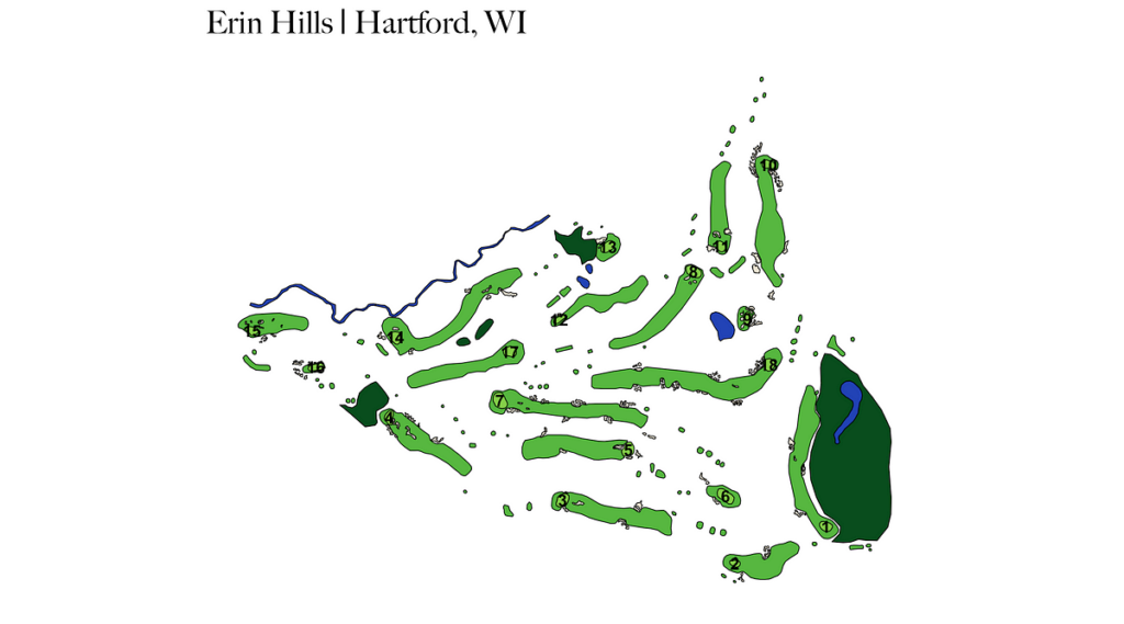
Plotting Golf Programs in R with Google Earth | by Adam Beaudet | Might, 2024
As soon as we’ve completed mapping our gap or course, it’s time to export all that tough work right into a KML file. This may be accomplished by clicking the three vertical dots on the left facet of the display screen the place your challenge resides. This challenge works finest with geoJSON knowledge, which we are able to simply convert our KML file to within the subsequent steps. Now we’re prepared to go to R.
The packages we might want to put together us for plotting are: sf (for working with geospatial knowledge), tidyverse (for knowledge cleansing and plotting), stringr (for string matching), and geojsonsf (for changing from KML to geoJSON). Our first step is studying within the KML file, which might be accomplished with the st_read() operate from sf.
# load libraries
library(sf)
library(tidyverse)
library(stringr)
library(geojsonsf)kml_df <- st_read("/Customers/adambeaudet/Downloads/erin_hills.kml")
Nice! Now we should always have our golf course KML knowledge in R. The info body ought to have 2 columns: Identify (challenge identify, or course identify in our case), and geometry (an inventory of all particular person factors comprising the polygons we traced). As briefly talked about earlier, let’s convert our KML knowledge to geoJSON and in addition extract the course identify and gap numbers.
# convert from KML to geoJSON
geojson_df <- st_as_sf(kml_df, "POLYGON")# extracting course identify and gap quantity from polygon identify
# assuming "course_hole_element" naming conference is used for polygons
geojson_df$course_name <- str_match(geojson_df$Identify, “^(.+)_hole”)[,2]
geojson_df$hole_num <- gsub(“.*_hole_(d+)_.*”, “1”, geojson_df$Identify)
To get our maps to level due north we have to challenge them in a means that preserves course. We are able to do that with the st_transform() operate.
# outline a CRS for therefore map at all times factors due north
crs <- "+proj=lcc +lat_1=33 +lat_2=45 +lat_0=39 +lon_0=-96 +x_0=0 +y_0=0 +datum=WGS84 +models=m +no_defs"# rework knowledge to CRS
geojson_df <- st_transform(geojson_df, crs)
We’re nearly able to plot, however first, we have to inform ggplot2 how every polygon needs to be coloured. Under is the colour palette my challenge is utilizing, however be happy to customise as you would like.
Non-compulsory: on this step we are able to additionally calculate the centroids of our polygons with the st_centroid() operate so we are able to overlay the outlet quantity onto every inexperienced.

geojson_df <- geojson_df %>%
mutate(coloration = case_when(
grepl(“_tee$”, Identify) ~ “#57B740”,
grepl(“_bunker$”, Identify) ~ “#EDE6D3”,
grepl(“_water$”, Identify) ~ “#2243b6”,
grepl(“_fairway$”, Identify) ~ “#57B740”,
grepl(“_green$”, Identify) ~ “#86D14A”,
grepl(“_hazard$”, Identify) ~ “#094d1d”
)) %>%
mutate(centroid = st_centroid(geometry))
We’re formally able to plot. We are able to use a mix of geom_sf(), geom_text(), and even geom_point() if we wish to get fancy and plot pictures on prime of our map. I usually take away gridlines, axis labels, and the legend for a cleaner look.
ggplot() +
geom_sf(knowledge = geojson_df, aes(fill = coloration), coloration = "black") +
geom_text(knowledge = filter(geojson_df, grepl("_green", Identify)),
aes(x = st_coordinates(centroid)[, 1],
y = st_coordinates(centroid)[, 2],
label = hole_num),
dimension = 3, coloration = "black", fontface = "daring", hjust = 0.5, vjust = 0.5) +
scale_fill_identity() +
theme_minimal() +
theme(axis.title.x = element_blank(),
axis.title.y = element_blank(),
axis.textual content.x = element_blank(),
axis.textual content.y = element_blank(),
plot.title = element_text(dimension = 16),
panel.grid.main = element_blank(),
panel.grid.minor = element_blank()) +
theme(legend.place = "none") +
labs(title = 'Erin Hills | Hartford, WI')
And there you’ve gotten it — a golf course plotted in R, what an idea!
To view different programs I’ve plotted on the time of writing this text, you possibly can go to my Shiny app: https://abodesy14.shinyapps.io/golfMapsR/
For those who adopted alongside, had enjoyable in doing so, or are intrigued, be happy to strive mapping your favourite programs and create a Pull Request for the golfMapsR repository that I preserve: https://github.com/abodesy14/golfMapsR
With some mixed effort, we are able to create a pleasant little database of plottable golf programs all over the world!