A Winding Highway to Parameter Effectivity | by Mariano Kamp | Jan, 2024

Let’s get began with our principal exercise.

The design selections left for us within the mannequin structure are sometimes expressed as hyperparameters. For LoRA particularly, we will outline which modules to adapt and how giant r must be for every module’s adapter.
Within the final article we solely instructed deciding on these modules based mostly on our understanding of the duty and the structure.

Now, we’ll dive deeper. The place ought to we apply finetuning in any respect?

Within the illustration above, you possibly can see all of the potential modules that we may finetune–together with the classifier and the embeddings–on the left. On the suitable, I’ve made a pattern choice for the illustration . However how can we arrive at an precise choice?
Let’s take a look at our choices from a excessive degree:

• Classifier
  It’s clear that we completely want to coach the classifier. It’s because it has not been skilled throughout pre-training and, therefore, for our finetuning, it’s randomly initialized. Moreover, its central place makes it extremely impactful on the mannequin efficiency, as all data should circulation by way of it. It additionally has probably the most instant influence on the loss calculation because it begins on the classifier. Lastly, it has few parameters, due to this fact, it’s environment friendly to coach.
  In conclusion, we all the time finetune the classifier, however don’t adapt it (with LoRA).
• Embeddings
  The embeddings reside on the backside–near the inputs–and carry the semantic which means of the tokens. That is necessary for our downstream process. Nonetheless, it’s not “empty”. Even with out finetuning, we’d get all of what was discovered throughout pre-training. At this level, we’re contemplating whether or not finetuning the embeddings straight would give us extra skills and if our downstream process would profit from a refined understanding of the token meanings?
  Let’s replicate. If this have been the case, may this extra data not even be discovered in one of many layers above the embeddings, maybe much more effectively?
  Lastly, the embeddings sometimes have numerous parameters, so we must adapt them earlier than finetuning.
  Taking each points collectively, we determined to go on this feature and never make the embeddings trainable (and consequently not apply LoRA to them).
• Transformer Layers
  Finetuning all parameters within the transformer layers can be inefficient. Subsequently, we have to no less than adapt them with LoRA to change into parameter-efficient. This leads us to think about whether or not we must always practice all layers, and all elements inside every layer? Or ought to we practice some layers, some elements, or particular combos of each?
  There isn’t a normal reply right here. We’ll adapt these layers and their modules and discover the main points additional on this article.

Within the illustration above, on the suitable, you possibly can see an exemplary collection of modules to finetune on the suitable. This is only one mixture, however many different combos are doable. Have in mind as properly that the illustration solely reveals 5 layers, whereas your mannequin possible has extra. As an example, the RoBERTa base mannequin–utilized in our instance–has 12 layers, a quantity that’s thought of small by in the present day’s requirements. Every layer additionally has 6 elements:

• Consideration: Question, Key, Worth, Output
• Feed Ahead: Up, Down

Even when we disregard that we additionally wish to tune r and — for now — simply give attention to the binary determination of which modules to incorporate, this can go away us with 64 (2**6) combos per layer. Given this solely appears on the combos of 1 layer, however that we’ve 12 layers that may be mixed, we find yourself with greater than a sextillion combos:

In [1]: (2**6)**12.
Out[1]: 4.722366482869645e+21

It’s straightforward to see that we can’t exhaustively compute all combos, not to mention to discover the area manually.

Sometimes in pc science, we flip to the cube once we wish to discover an area that’s too giant to completely examine. However on this case, we may pattern from that area, however how would we interpret the outcomes? We might get again quite a lot of arbitrary mixture of layers and elements (no less than 12*6=72 following the small instance of above). How would we generalize from these particulars to search out higher-level guidelines that align with our pure understanding of the issue area? We have to align these particulars with our conceptual understanding on a extra summary degree.

Therefore, we have to think about teams of modules and search for constructions or patterns that we will use in our experiments, slightly than working on a set of particular person elements or layers. We have to develop an instinct about how issues ought to work, after which formulate and check hypotheses.

Query: Does it assist to experiment on outlined teams of parameters in isolation? The reply is sure. These remoted teams of parameters can cleared the path regardless that we might have to mix a few of them later to attain one of the best outcomes. Testing in isolation permits us to see patterns of influence extra clearly.

Nonetheless, there’s a threat. When these patterns are utilized in mixture, their influence could change. That’s not good, however let’s not be so unfavourable about it 🙂 We have to begin someplace, after which refine our method if wanted.

Prepared? Let’s do this out.

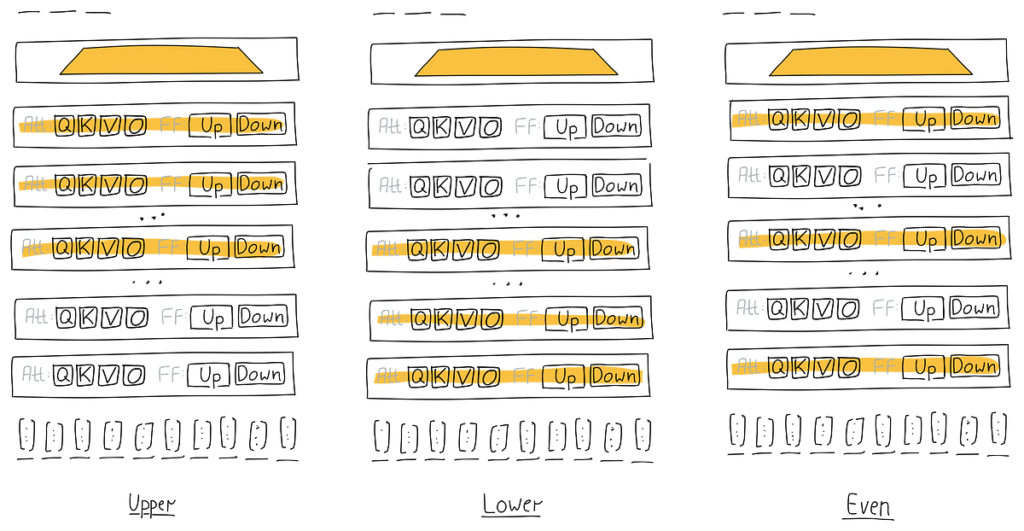
Tuning Vertically / Layer-wise

I believe that the higher layers, nearer to the classification head, will likely be extra impactful than the decrease layers. Right here is my considering: Our process is sentiment evaluation. It could make sense, wouldn’t it, that many of the particular selections should be made both within the classification head or near it? Like recognizing sure phrases (“I wanted that like a gap in my head”) or composed constructs (“The check-in expertise negated the in any other case great service”). This might counsel that it’s essential to finetune the parameters of our community that outline how totally different tokens are used collectively–in context–to create a sentiment versus altering the which means of phrases (within the embeddings) in comparison with their which means in the course of the pre-training.

Even when that’s not all the time the case, adapting the higher layers nonetheless supplies the chance to override or refine selections from the decrease layers and the embeddings. Then again, this implies that finetuning the decrease layers is much less necessary.

That sounds like a strong speculation to check out (Oops. Message from future Mariano: Don’t cease studying right here).

As an apart, we’re not reflecting on the overall necessity of the embeddings or any of the transformer layers. That call has already been made: all of them have been a part of the pre-training and will likely be a part of our finetuned mannequin. What we’re contemplating at this level is how we will greatest assist the mannequin study our downstream process, which is sentiment evaluation. The query we’re asking is: which weights ought to we finetune for influence and to attain parameter effectivity?

Let’s put this to the check.

To obviously see the impact of our speculation, what can we check it towards? Let’s design experiments that ought to exaggerate the impact:

• In our first experiment we finetune and adapt all elements of the higher half of the mannequin, particularly layers 7–12 in our instance. That is our speculation.
• In distinction, we run one other experiment the place we solely finetune the layers within the decrease half of the mannequin. Particularly, we practice layers 1–6 with all elements. That’s the other of our speculation.
• Let’s think about one other contrastive speculation as properly: {that a} gentle contact to all layers is extra useful than simply tuning the highest layers. So, let’s additionally embody a 3rd situation the place we finetune half of the layers however unfold them out evenly.
• Let’s additionally embody an experiment the place we tune all layers (not depicted within the illustration above). This isn’t a good efficiency comparability as we practice twice as many parameters as within the first three experiments. Nonetheless, for that motive, it highlights how a lot efficiency we doubtlessly lose within the earlier situations the place we have been tuning solely half the variety of parameters.

In abstract, we’ve 3+1 situations that we wish to run as experiments. Listed below are the outcomes:

Execution of Experiments:

We begin by utilizing the already tuned studying charge, epochs. Then, we run trials (coaching runs) with totally different values for the situation settings, corresponding to decrease, higher, even, all. Inside AMT, we run these experiments as a Grid Search.

Query: Grid Search is thought to be easy, however inefficient to find one of the best resolution. So why are we utilizing it?

Let’s take a step again. If we have been to run just a few trials with Bayesian Search, we’d rapidly study hyperparameter values which might be performing properly. This might bias the next trials to give attention to these values, i.e., pre-dominantly keep nearer to identified good values. Whereas more and more exploiting what we study in regards to the search area is an efficient technique to search out one of the best values, its bias makes it obscure the explored area, as we under-sample in areas that confirmed low efficiency early on.

With Grid Search, we will exactly outline which parameter values to discover, making the outcomes simpler to interpret.

Actually, if you happen to have been to take a look at the supplied code, you’d see that AMT would reject sampling the identical values greater than as soon as. However we would like that, therefore, we introduce a dummy variable with values from 0 to the variety of trials we wish to conduct. That is useful, permitting us to repeat the trials with the identical hyperparameter values to estimate the usual deviation of this mixture.

Whereas we used 5 trials every for an already tuned baseline situation above to see how properly we will reproduce a selected mixture of hyperparameter values, right here we use 7 trials per mixture to get a barely extra exact understanding of this mixture’s variance to see tiny variations.

The identical rules are utilized to the next two situations on this article and won’t be talked about once more henceforth.

Let’s get the simple factor out of the way in which first: As anticipated, tuning all layers and consequently utilizing double the variety of parameters, improves efficiency probably the most. This enchancment is obvious within the backside determine.
Additionally, the peaks of all situations, as proven within the density plots on the suitable of the person figures, are comparatively shut. When evaluating these peaks, which signify probably the most ceaselessly noticed efficiency, we solely see an enchancment of ~0.08 in validation accuracy between the worst and greatest situation. That’s not a lot. Subsequently, we think about it a wash.

Regardless, let’s nonetheless study our authentic speculation: We (me, actually) anticipated that finetuning the higher six layers would yield higher efficiency than finetuning the decrease six layers. Nonetheless, the information disagrees. For this process it makes no distinction. Therefore, I must replace my understanding.

Now we have two potential takeaways:

• Spreading the layers evenly is slightly higher than specializing in the highest or backside layers. That mentioned, the development is so small that this perception could also be brittle and won’t generalize properly, not occasion to new runs of the identical mannequin. Therefore, we’ll discard our “discovery”.
• Tuning all layers, with double the associated fee, produces marginally higher outcomes. This consequence, nevertheless, is no surprise anybody. Nonetheless good to see confirmed although, as we in any other case would have discovered a possibility to save lots of trainable parameters, i.e., price.

Total, good to know all of that, however as we don’t think about it actionable, we’re shifting on. In case you are , you could find extra particulars on this notebook.

Tuning Horizontally / Element-wise

Inside every transformer layer, we’ve 4 discovered projections used for consideration that may be tailored throughout finetuning:

• Q — Question, 768 -> 768
• Okay — Key, 768 -> 768
• V — Worth, 768 -> 768
• O — Output, 768 -> 768

Along with these, we use two linear modules in every position-wise feedforward layer that dwell throughout the similar transformer layer because the projections from above:

• Up — Up projection, 768 -> 3072
• Down — Down projection, 3072 -> 768

We will already see from the numbers above that the feedforward layers (ff) are 4 occasions as giant because the QKVO projections we beforehand mentioned. Therefore the ff elements could have a doubtlessly bigger influence and positively increased price.

In addition to this, what different expectations may we’ve? It’s onerous to say. We all know from Multi-Question Consideration [3] that the question projection is especially necessary, however does this significance maintain when finetuning with an adapter on our process (versus, for instance, pre-training)? As an alternative, let’s check out what the influence of the person elements is and proceed based mostly on these outcomes. We can see which elements are the strongest and possibly this can enable us to only decide these for tuning going ahead.

Let’s run these experiments and examine the outcomes:

As was to be anticipated, the ff layers use their four-times measurement benefit to outperform the eye projections. Nonetheless, we will see that there are variations inside these two teams. These variations are comparatively minor, and if you wish to leverage them, it’s essential to validate their applicability in your particular process.

An necessary statement is that by merely tuning one of many ff layers (~0.943), we may nearly obtain the efficiency of tuning all modules from the “LoRA Base” situation (~0.946). Consequently, if we’re seeking to steadiness between total efficiency and the parameter depend, this could possibly be a great technique. We’ll hold this in thoughts for the ultimate comparability.

Inside the consideration projections (center determine) it seems that the question projection didn’t show as impactful as anticipated. Contrarily, the output and worth projections proved extra helpful. Nonetheless, on their very own, they weren’t that spectacular.

To date, we’ve appeared on the particular person contributions of the elements. Let’s additionally examine if their influence overlaps or if combining elements can enhance the outcomes.

Let’s run a number of the doable combos and see if that is informative. Listed below are the outcomes:

Trying on the numbers charted above the primary takeaway is that we’ve no efficiency regressions. On condition that we added extra parameters and mixed current combos, that’s the way it must be. Nonetheless, there may be all the time the possibility that when combining design selections their mixed efficiency is worse than their particular person efficiency. Not right here although, good!

We must always not over-interpret the outcomes, however it’s attention-grabbing to acknowledge that once we testing our speculation individually the output projection’s efficiency was barely forward of the efficiency of the worth projection. Right here now, together with the position-wise feed ahead up projection this relationship is reversed (now: o+up ~0.945, v+up ~0.948).

We’ll additionally acknowledge within the earlier experiment, that the up projection was already performing nearly on that degree by itself. Subsequently, we hold our enthusiasm in examine, however embody this situation in our remaining comparability. If solely, as a result of we get a efficiency that’s barely higher than when tuning and adapting all elements in all layers, “LoRA Base”, however with a lot fewer parameters.

You’ll find extra particulars on this notebook.

We all know from the literature [2] that it is strongly recommended to make use of a small r worth, which means that r is barely a fraction of the minimal dimension of the unique module, e.g. to make use of 8 as an alternative of 768. Nonetheless, let’s validate this for ourselves and get some empirical suggestions. May it’s price investigating utilizing a bigger worth for r, regardless of the standard knowledge?

For the earlier trials, we used r=8 and invested extra time to tune learning-rate and the variety of epochs to coach for this worth. Now attempting totally different values for r will considerably alter the capability of the linear modules. Ideally, we’d re-tune the learning-rate for every worth of r, however we goal to be frugal. Consequently, for now, we follow the identical learning-rate. Nonetheless, as farther we go away from our tuned r=8worth as stronger the necessity to retune the opposite hyperparameters talked about above.
A consideration we have to keep in mind when reviewing the outcomes:

Within the first determine, we see that the mannequin efficiency is just not significantly delicate to extra capability with good performances at r=4 and r=8. r=16was a tiny bit higher, however can also be dearer when it comes to parameter depend. So let’s hold r=4 and r=8 in thoughts for our remaining comparability.
To see the impact of r on the parameter depend, we may also embody r=1 within the remaining comparability.

One odd factor to look at within the figures above is that the efficiency is falling off sharply at r=32. Offering a mannequin, that makes use of residual connections, extra capability ought to yield the identical or higher efficiency than with a decrease capability. That is clearly not the case right here. However as we tuned the learning-rate for r=8 and we now have many extra learnable parameters with r=32 (see the higher proper panel in previous determine) we also needs to cut back the learning-rate, or ideally, re-tune the learning-rate and variety of epochs to adapt to the a lot bigger capability. Trying on the decrease proper panel within the earlier determine we must always then additionally think about including extra regularization to take care of the extra pronounced overfitting we see.

Regardless of the overall potential for enchancment when offering the mannequin with extra capability, the opposite values of r we noticed didn’t point out that extra capability would enhance efficiency with out additionally markedly growing the variety of parameters. Subsequently, we’ll skip chasing an excellent bigger r.

Extra particulars on this notebook.

All through this lengthy article, we’ve gathered quite a few analytical outcomes. To consolidate these findings, let’s discover and evaluate a number of attention-grabbing combos of hyperparameter values in a single place. For our functions, a result’s thought of attention-grabbing if it both improves the general efficiency of the mannequin or provides us extra insights about how the mannequin works to in the end strengthen our intuitive understanding

All experiments finetune the sst2 process on RoBERTa base as seen within the RoBERTa paper [1].

Execution of Experiments:

As earlier than, after I present the outcomes of a situation (reported because the “target_tuner_name” column within the desk above, and as labels on the y-axis within the graph), it’s based mostly on executing the similar mixture of hyperparameter values 5 occasions. This permits me to report the imply and commonplace deviation of the target metric.

Now, let’s focus on some observations from the situations depicted within the graph above.

Classifier Solely

This baseline—the place we solely practice the classifier head—has the bottom price. Check with parameters_relative, which signifies the proportion of parameters wanted, in comparison with a full finetuning. That is illustrated within the second panel, exhibiting that ~0.5% is the bottom parameter depend of all situations.

This has a useful influence on the “GPU Reminiscence” panel (the place decrease is best) and markedly within the “Prepare Velocity” panel (the place increased is best). The latter signifies that this situation is the quickest to coach, due to the decrease parameter depend, and in addition as a result of there are fewer modules to deal with, as we don’t add extra modules on this situation.

This serves as an informative bare-bones baseline to see relative enhancements in coaching velocity and GPU reminiscence use, but in addition highlights a tradeoff: the mannequin efficiency (first panel) is the bottom by a large margin.
Moreover, this situation reveals that 0.48% of the total fine-tuning parameters signify the minimal parameter depend. We allocate that fraction of the parameters solely for the classifier. Moreover, as all different situations tune the classifier, we constantly embody that 0.48% along with no matter parameters are additional tuned in these situations.

LoRA Base

This situation serves as the muse for all experiments past the baselines. We user=8 and adapt and finetune all linear modules throughout all layers.

We will observe that the mannequin efficiency matches the total finetuning efficiency. We’d have been fortunate on this case, however the literature counsel that we will anticipate to just about match the total finetuning efficiency with nearly 1% of the parameters. We will see proof of this right here.

Moreover, due to adapting all linear modules, we see that the practice velocity is the bottom of all experiments and the GPU reminiscence utilization is amongst the best, however in keeping with many of the different situations.

LoRA all, r={1,4,8}

Total, these situations are variations of “LoRA Base” however with totally different values of r. There may be solely a small distinction within the efficiency. Nonetheless, as anticipated, there’s a constructive correlation between r and the parameter depend and a barely constructive correlation between r and GPU reminiscence utilization. Regardless of the latter, the worth of r stays so low that this doesn’t have a considerable influence on the underside line, particularly the GPU reminiscence utilization. This confirms what we explored within the authentic experiments, component-wise, as mentioned above.

When reviewing r=1, nevertheless, we see that it is a particular case. With 0.61% for the relative parameter depend, we’re only a smidgen above the 0.48% of the “Classifier Solely” situation. However we see a validation accuracy of ~0.94 with r=1, in comparison with ~0.82 with “Classifier Solely”. With simply 0.13% of the whole parameters, tailored solely within the transformer layers, we will elevate the mannequin’s validation accuracy by ~0.12. Bam! That is spectacular, and therefore, if we’re excited about a low parameter depend, this could possibly be our winner.

Concerning GPU reminiscence utilization, we’ll evaluate this a bit later. However briefly, in addition to allocating reminiscence for every parameter within the mannequin, the optimizer, and the gradients, we additionally must hold the activations round to calculate the gradients throughout backpropagation.

Moreover, bigger fashions will present a much bigger influence of selecting a small worth for r.

For what it’s price, the situation “LoRA all, r=8” used an identical hyperparameter values to “LoRA Base”, however was executed independently. To make it simpler to check r=1, r=4 and r=8, this situation was nonetheless evaluated.

LoRA ff_u

On this situation we’re tuning solely the position-wise feed ahead up projections, throughout all layers. This results in a discount in each the variety of parameters and the variety of modules to adapt. Consequently, the information reveals an enchancment in coaching velocity and a discount in GPU reminiscence utilization.

However we additionally see a small efficiency hit. For “LoRA Base” we noticed ~0.946, whereas on this situation we solely see ~0.942, a drop of ~0.04.

Particulars on the comparisons on this notebook.

When trying on the GPU reminiscence panel above, two issues change into apparent:

One — LoRA, by itself, doesn’t dramatically cut back the reminiscence footprint

That is very true when we adapt small fashions like RoBERTa base with its 125M parameters.

Within the previous article’s part on intrinsic dimensionality, we discovered that for present technology fashions (e.g., with 7B parameters), absolutely the worth of r will be even smaller than for smaller capability fashions. Therefore, the memory-saving impact will change into extra pronounced with bigger fashions.

Moreover utilizing LoRA makes utilizing quantization simpler and extra environment friendly – an ideal match. With LoRA, solely a small proportion of parameters should be processed with excessive precision: It’s because we replace the parameters of the adapters, not the weights of the unique modules. Therefore, the vast majority of the mannequin weights will be quantized and used at a lot decrease precision.

Moreover, we sometimes use AdamW as our optimizer. Not like SGD, which tracks solely a single world studying charge, AdamW tracks shifting averages of each the gradients and the squares of the gradients for every parameter. This means that for every trainable parameter, we have to hold observe of two values, which may doubtlessly be in FP32. This course of will be fairly pricey. Nonetheless, as described within the earlier paragraph, when utilizing LoRA, we solely have just a few parameters which might be trainable. This could considerably cut back the associated fee, in order that we will use the sometimes parameter-intensive AdamW, even with giant r values.

We could look into these points partially 4 of our article sequence, given sufficient curiosity of you, pricey reader.

Two–GPU reminiscence utilization is barely not directly correlated with parameter depend

Wouldn’t it’s nice if there was a direct linear relationship between the parameter depend and the wanted GPU reminiscence? Sadly there are a number of findings within the diagrams above that illustrate that it isn’t that straightforward. Let’s discover out why.

First we have to allocate reminiscence for the mannequin itself, i.e., storing all parameters. Then, for the trainable parameters, we additionally must retailer the optimizer state and gradients (for every trainable parameter individually). As well as we have to think about reminiscence for the activations, which not solely relies on the parameters and layers of the mannequin, but in addition on the enter sequence size. Plus, it’s essential to do not forget that we have to keep these activations from the ahead go as a way to apply the chain rule in the course of the backward go to do backpropagation.

If, throughout backpropagation, we have been to re-calculate the activations for every layer when calculating the gradients for that layer, we’d not keep the activations for therefore lang and will save reminiscence at the price of elevated computation.

This method is named gradient checkpointing. The quantity of reminiscence that may be saved relies on how a lot extra reminiscence for activations must be retained. It’s necessary to do not forget that backpropagation includes repeatedly making use of the chain rule, step-by-step, layer by layer:

Recap — Chain Rule throughout Again Propagation

Throughout backpropagation, we calculate the error on the high of the community (within the classifier) after which propagate the error again to all trainable parameters that have been concerned. These parameters are adjusted based mostly on their contributions to the error, to do higher sooner or later. We calculate the parameters’ contributions by repeatedly making use of the chain rule, begin on the high and traversing the computation graph in direction of the inputs. That is essential as a result of any change in a parameter on a decrease layer can doubtlessly influence the parameters in all of the layers above.

To calculate the native gradients (for every step), we might have the values of the activations for all of the steps between the respective trainable parameter and the highest (the loss perform which is utilized on the classification head). Thus, if we’ve a parameter in one of many high layers (near the pinnacle), we have to keep fewer activations in comparison with when coaching a parameter within the decrease layers. For these decrease layer parameters, we have to traverse a for much longer graph to succeed in the classification head and, therefore, want to keep up extra reminiscence to maintain the activations round.

In our particular mannequin and process, you possibly can see the impact illustrated beneath. We practice a person mannequin for every layer, through which solely that specific layer undergoes coaching. This fashion, we will isolate the impact of the layer’s relative place. We then plot the quantity of GPU reminiscence required for every mannequin, and due to this fact for every layer, throughout coaching.

Within the graph beneath (see left panel) you possibly can see that if we’re nearer to the underside of the mannequin (i.e., low layer quantity) the GPU reminiscence requirement is decrease than if we’re near the highest of the mannequin (i.e., excessive layer quantity) the place the loss originates.

With gradient checkpointing enabled (see proper panel), we now not can acknowledge this impact. As an alternative of saving the activations till backprop we re-calculate them when wanted. Therefore, the distinction in reminiscence utilization between the left and proper panel are the activations that we keep for the backward go.

Execution of Experiments:

As with earlier experiments, I used AMT with Grid Search to offer unbiased outcomes.

It is very important keep in mind, that recalculating the activations throughout backpropagation is sluggish, so we’re buying and selling of computational velocity with reminiscence utilization.

Extra particulars on the testing will be discovered on this notebook.

As an apart, to one of the best of my understanding, utilizing Gradient Checkpointing ought to solely have non-functional influence. Sadly, this isn’t what I’m seeing although (issue). I could also be misunderstanding methods to use Hugging Face’s Transformers library. If anybody has an concept why this can be the case, please let me know.
Consequently, take the graphs from above with a little bit of warning.

We could revisit the subject of reminiscence partially 4 of this text sequence, though it’s not strictly a LoRA matter. In case you’re , please let me know within the feedback beneath.