Develop Your First AI Agent: Deep Q-Studying | by Heston Vaughan | Dec, 2023

1. Preliminary Setup

Earlier than we begin coding our AI agent, it is suggested that you’ve a strong understanding of Object Oriented Programming (OOP) ideas in Python.

In the event you don’t have Python put in already, beneath is a straightforward tutorial by Bhargav Bachina to get you began. The model I might be utilizing is 3.11.6.

The one dependency you’ll need is TensorFlow, an open-source machine studying library by Google that we’ll use to construct and prepare our neural community. This may be put in by means of pip within the terminal. My model is 2.14.0.

pip set up tensorflow

Or if that doesn’t work:

pip3 set up tensorflow

Additionally, you will want the bundle NumPy, however this ought to be included with TensorFlow. In the event you run into points there, pip set up numpy.

It is usually advisable that you simply create a brand new file for every class, (e.g., setting.py). This may hold you from being overwhelmed and ease troubleshooting any errors you might run into.

To your reference, right here is the GitHub repository with the finished code: https://github.com/HestonCV/rl-gym-from-scratch. Be at liberty to clone, discover, and use it as a reference level!

2. The Huge Image

To essentially perceive the ideas fairly than simply copying code, it’s essential to get a deal with on the completely different components we’re going to construct and the way they match collectively. This fashion, each bit can have a spot within the larger image.

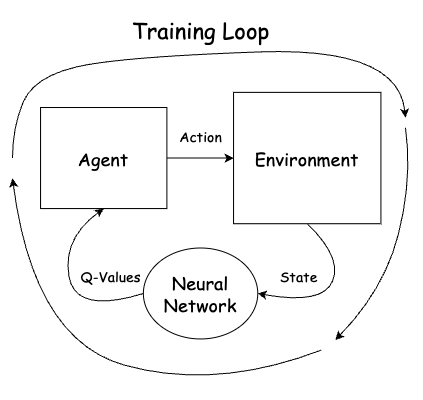
Under is the code for one coaching loop with 5000 episodes. An episode is basically one full spherical of interplay between the agent and the setting, from begin to end.

This shouldn’t be carried out or totally understood at this level. As we construct out every half, if you wish to see how a selected class or technique might be used, refer again to this.

from setting import Atmosphere
from agent import Agent
from experience_replay import ExperienceReplay
import time
if __name__ == '__main__':
grid_size = 5
setting = Atmosphere(grid_size=grid_size, render_on=True)
agent = Agent(grid_size=grid_size, epsilon=1, epsilon_decay=0.998, epsilon_end=0.01)
# agent.load(f'fashions/model_{grid_size}.h5')
experience_replay = ExperienceReplay(capability=10000, batch_size=32)
# Variety of episodes to run earlier than coaching stops
episodes = 5000
# Max variety of steps in every episode
max_steps = 200
for episode in vary(episodes):
# Get the preliminary state of the setting and set carried out to False
state = setting.reset()
# Loop till the episode finishes
for step in vary(max_steps):
print('Episode:', episode)
print('Step:', step)
print('Epsilon:', agent.epsilon)
# Get the motion alternative from the brokers coverage
motion = agent.get_action(state)
# Take a step within the setting and save the expertise
reward, next_state, carried out = setting.step(motion)
experience_replay.add_experience(state, motion, reward, next_state, carried out)
# If the expertise replay has sufficient reminiscence to offer a pattern, prepare the agent
if experience_replay.can_provide_sample():
experiences = experience_replay.sample_batch()
agent.be taught(experiences)
# Set the state to the next_state
state = next_state
if carried out:
break
# time.sleep(0.5)
agent.save(f'fashions/model_{grid_size}.h5')

Every inside loop is taken into account one step.

In every step:

• The state is retrieved from the setting.
• The agent chooses an motion based mostly on this state.
• Atmosphere is acted on, returning the reward, ensuing state after taking the motion, and whether or not the episode is completed.
• The preliminary state, motion, reward, next_state, and carried out are then saved into experience_replay as a form of long-term reminiscence (expertise).
• The agent is then skilled on a random pattern of those experiences.

On the finish of every episode, or nevertheless typically you prefer to, the mannequin weights are saved to the fashions folder. These can later be preloaded to maintain from coaching from scratch every time. The setting is then reset firstly of the subsequent episode.

This primary construction is just about all it takes to create an clever agent to resolve a big number of issues!

As acknowledged within the introduction, our drawback for the agent is sort of easy: get from its preliminary place in a grid to the designated aim place.

3. The Atmosphere: Preliminary Foundations

The obvious place to start out in growing this method is the setting.

To have a functioning RL gymnasium, the setting must do a couple of issues:

• Keep the present state of the world.
• Preserve monitor of the aim and agent.
• Permit the agent to make adjustments to the world.
• Return the state in a kind the mannequin can perceive.
• Render it in a approach we are able to perceive to look at the agent.

This would be the place the agent spends its total life. We are going to outline the setting as a easy sq. matrix/2D array, or a listing of lists in Python.

This setting can have a discrete state-space, that means that the attainable states the agent can encounter are distinct and countable. Every state is a separate, particular situation or state of affairs within the setting, in contrast to a steady state area the place the states can differ in an infinite, fluid method — consider chess versus controlling a automotive.

DQL is particularly designed for discrete action-spaces (a finite variety of actions)— that is what we might be specializing in. Different strategies are used for steady action-spaces.

Within the grid, empty area might be represented by 0s, the agent might be represented by a 1, and the aim might be represented by a -1. The dimensions of the setting might be no matter you prefer to, however because the setting grows bigger, the set of all attainable states (state-space) grows exponentially. This may sluggish coaching time considerably.

The grid will look one thing like this when rendered:

[0, 1, 0, 0, 0]
[0, 0, 0, 0, 0]
[0, 0, 0, 0, 0]
[0, 0, 0, -1, 0]
[0, 0, 0, 0, 0]

Setting up the Atmosphere class and reset technique
We are going to start by implementing the Atmosphere class and a method to initialize the setting. For now, it should take an integer, grid_size, however we’ll increase on this shortly.

import numpy as np
class Atmosphere:
def __init__(self, grid_size):
self.grid_size = grid_size
self.grid = []
def reset(self):
# Initialize the empty grid as a second listing of 0s
self.grid = np.zeros((self.grid_size, self.grid_size))

When a brand new occasion is created, Atmosphere saves grid_size and initializes an empty grid.

The reset technique populates the grid utilizing np.zeros((self.grid_size, self.grid_size)) , which takes a tuple, form, and outputs a 2D NumPy array of that form consisting solely of zeros.

A NumPy array is a grid-like information construction that behaves much like a listing in Python, besides that it permits us to effectively retailer and manipulate numerical information. It permits for vectorized operations, that means that operations are robotically utilized to all components within the array with out the necessity for express loops.

This makes computations on massive datasets a lot quicker and extra environment friendly in comparison with commonplace Python lists. Not solely that, however it’s the information construction that our agent’s neural community structure will count on!

Why the identify reset? Nicely, this technique might be known as to reset the setting and can ultimately return the preliminary state of the grid.

Including the agent and aim
Subsequent, we’ll assemble the strategies for including the agent and the aim to the grid.

import random
def add_agent(self):
# Select a random location
location = (random.randint(0, self.grid_size - 1), random.randint(0, self.grid_size - 1))
# Agent is represented by a 1
self.grid[location[0]][location[1]] = 1
return location
def add_goal(self):
# Select a random location
location = (random.randint(0, self.grid_size - 1), random.randint(0, self.grid_size - 1))
# Get a random location till it isn't occupied
whereas self.grid[location[0]][location[1]] == 1:
location = (random.randint(0, self.grid_size - 1), random.randint(0, self.grid_size - 1))
# Objective is represented by a -1
self.grid[location[0]][location[1]] = -1
return location

The places for the agent and the aim might be represented by a tuple (x, y). Each strategies choose random values inside the boundaries of the grid and return the situation. The principle distinction is that add_goal ensures it doesn’t choose a location already occupied by the agent.

We place the agent and aim at random beginning places to introduce variability in every episode, which helps the agent be taught to navigate the setting from completely different beginning factors, fairly than memorizing one route.

Lastly, we’ll add a way to render the world within the console to allow us to see the interactions between the agent and setting.

def render(self):
# Convert to a listing of ints to enhance formatting
grid = self.grid.astype(int).tolist()
for row in grid:
print(row)
print('') # So as to add some area between renders for every step

render does three issues: casts the weather of self.grid to sort int, converts it right into a Python listing, and prints every row.

The one cause we don’t print every row from the NumPy array instantly is just that it simply doesn’t look as good.

Tying all of it collectively..

import numpy as np
import random
class Atmosphere:
def __init__(self, grid_size):
self.grid_size = grid_size
self.grid = []
def reset(self):
# Initialize the empty grid as a second array of 0s
self.grid = np.zeros((self.grid_size, self.grid_size))
def add_agent(self):
# Select a random location
location = (random.randint(0, self.grid_size - 1), random.randint(0, self.grid_size - 1))
# Agent is represented by a 1
self.grid[location[0]][location[1]] = 1
return location
def add_goal(self):
# Select a random location
location = (random.randint(0, self.grid_size - 1), random.randint(0, self.grid_size - 1))
# Get a random location till it isn't occupied
whereas self.grid[location[0]][location[1]] == 1:
location = (random.randint(0, self.grid_size - 1), random.randint(0, self.grid_size - 1))
# Objective is represented by a -1
self.grid[location[0]][location[1]] = -1
return location
def render(self):
# Convert to a listing of ints to enhance formatting
grid = self.grid.astype(int).tolist()
for row in grid:
print(row)
print('') # So as to add some area between renders for every step
# Check Atmosphere
env = Atmosphere(5)
env.reset()
agent_location = env.add_agent()
goal_location = env.add_goal()
env.render()
print(f'Agent Location: {agent_location}')
print(f'Objective Location: {goal_location}')

>>>
[0, 0, 0, 0, 0]
[0, 0, -1, 0, 0]
[0, 0, 0, 0, 0]
[0, 0, 0, 1, 0]
[0, 0, 0, 0, 0]
Agent Location: (3, 3)
Objective Location: (1, 2)

When wanting on the places it might appear there was some error, however they need to be learn as (row, column) from the highest left to the underside proper. Additionally, do not forget that the coordinates are zero listed.

Okay, so the setting is outlined. What subsequent?

Increasing on reset
Let’s edit the reset technique to deal with inserting the agent and aim for us. Whereas we’re at it, let’s automate render as properly.

class Atmosphere:
def __init__(self, grid_size, render_on=False):
self.grid_size = grid_size
self.grid = []
# Make sure that so as to add the brand new attributes
self.render_on = render_on
self.agent_location = None
self.goal_location = None
def reset(self):
# Initialize the empty grid as a second array of 0s
self.grid = np.zeros((self.grid_size, self.grid_size))
# Add the agent and the aim to the grid
self.agent_location = self.add_agent()
self.goal_location = self.add_goal()
if self.render_on:
self.render()

Now, when reset is named, the agent and aim are added to the grid, their preliminary places are saved, and if render_on is ready to true it should render the grid.

...
# Check Atmosphere
env = Atmosphere(5, render_on=True)
env.reset()
# Now to entry agent and aim location you need to use Atmosphere's attributes
print(f'Agent Location: {env.agent_location}')
print(f'Objective Location: {env.goal_location}')

>>>
[0, 0, 0, 0, 0]
[0, 0, 0, 0, 0]
[0, 0, 0, 0, 0]
[0, 0, 0, 0, -1]
[1, 0, 0, 0, 0]
Agent Location: (4, 0)
Objective Location: (3, 4)

Defining the state of the setting
The final technique we’ll implement for now could be get_state. At first look it appears the state would possibly merely be the grid itself, however the issue with this method is it isn’t what the neural community will count on.

Neural networks usually want one-dimensional enter, not the two-dimensional form that grid at the moment is represented by. We are able to repair this by flattening the grid utilizing NumPy’s built-in flatten technique. This may place every row into the identical array.

def get_state(self):
# Flatten the grid from second to 1d
state = self.grid.flatten()
return state

This may remodel:

[0, 0, 0, 0, 0]
[0, 0, 0, 1, 0]
[0, 0, 0, 0, 0]
[0, 0, 0, 0, -1]
[0, 0, 0, 0, 0]

Into:

[0, 0, 0, 0, 0, 0, 0, 0, 1, 0, 0, 0, 0, 0, 0, 0, 0, 0, 0, -1, 0, 0, 0, 0, 0]

As you’ll be able to see, it’s not instantly apparent which cells are which, however this might be no drawback for a deep neural community.

Now we are able to replace reset to return the state proper after grid is populated. Nothing else will change.

def reset(self):
...
# Return the preliminary state of the grid
return self.get_state()

Full code up so far..

import random
class Atmosphere:
def __init__(self, grid_size, render_on=False):
self.grid_size = grid_size
self.grid = []
self.render_on = render_on
self.agent_location = None
self.goal_location = None
def reset(self):
# Initialize the empty grid as a second array of 0s
self.grid = np.zeros((self.grid_size, self.grid_size))
# Add the agent and the aim to the grid
self.agent_location = self.add_agent()
self.goal_location = self.add_goal()
if self.render_on:
self.render()
# Return the preliminary state of the grid
return self.get_state()
def add_agent(self):
# Select a random location
location = (random.randint(0, self.grid_size - 1), random.randint(0, self.grid_size - 1))
# Agent is represented by a 1
self.grid[location[0]][location[1]] = 1
return location
def add_goal(self):
# Select a random location
location = (random.randint(0, self.grid_size - 1), random.randint(0, self.grid_size - 1))
# Get a random location till it isn't occupied
whereas self.grid[location[0]][location[1]] == 1:
location = (random.randint(0, self.grid_size - 1), random.randint(0, self.grid_size - 1))
# Objective is represented by a -1
self.grid[location[0]][location[1]] = -1
return location
def render(self):
# Convert to a listing of ints to enhance formatting
grid = self.grid.astype(int).tolist()
for row in grid:
print(row)
print('') # So as to add some area between renders for every step
def get_state(self):
# Flatten the grid from second to 1d
state = self.grid.flatten()
return state

You’ve got now efficiently carried out the muse for the setting! Though, for those who haven’t seen, we are able to’t work together with it but. The agent is caught in place.

We are going to return to this drawback later after the Agent class has been coded to offer higher context.

4. Implement The Agent Neural Structure and Coverage

As acknowledged beforehand, the agent is the entity that’s given the state of its setting, on this case a flattened model of the world grid, and comes to a decision on what motion to take from the action-space.

Simply to reiterate, the action-space is the set of all attainable actions, on this state of affairs the agent can transfer up, down, left, and proper, so the scale of the motion area is 4.

The state-space is the set of all attainable states. This generally is a large quantity relying on the setting and perspective of the agent. In our case, if the world is a 5×5 grid there are 600 attainable states, but when the world is a 25×25 grid there are 390,000, wildly rising the coaching time.

For an agent to successfully be taught to finish a aim it wants a couple of issues:

• Neural community to approximate the Q-values (estimated complete quantity of future reward for an motion) within the case of DQL.
• Coverage or a technique that the agent follows to decide on an motion.
• Reward alerts from the setting to inform an agent how properly it’s doing.
• Capacity to coach on previous experiences.

There are two completely different insurance policies one can implement:

• Grasping Coverage: Select the motion with the very best Q-value within the present state.
• Epsilon-Grasping Coverage: Select the motion with the very best Q-value within the present state, however there’s a small probability, epsilon (generally denoted as ϵ), to decide on a random motion. If epsilon = 0.02 then there’s a 2% probability that the motion might be random.

What we’ll implement is the Epsilon-Grasping Coverage.

Why would random actions assist the agent be taught? Exploration.

When the agent begins, it might be taught a suboptimal path to the aim and proceed to make this alternative with out ever altering or studying a brand new route.

Starting with a big epsilon worth and slowly lowering it permits the agent to completely discover the setting because it updates its Q-values earlier than exploiting the discovered methods. The quantity we lower epsilon by over time is named epsilon decay, which is able to make extra sense quickly.

Like we did with the setting, we’ll symbolize the agent with a category.

Now, earlier than we implement the coverage, we’d like a method to get Q-values. That is the place our agent’s mind — or neural community — is available in.

The neural community
With out getting too off monitor right here, a neural community is just an enormous operate. The values go in, get handed to every layer and reworked, and a few completely different values come out on the finish. Nothing greater than that. The magic is available in when coaching begins.

The concept is to provide the NN massive quantities of labeled information like, “right here is an enter, and here’s what it’s best to output”. It slowly adjusts the values between neurons with every coaching step, making an attempt to get as shut as attainable to the given outputs, discovering patterns inside the information, and hopefully serving to us predict for inputs the community has by no means seen.

The Agent class and defining the neural structure
For now we’ll outline the neural structure utilizing TensorFlow and deal with the “ahead move” of the info.

from tensorflow.keras.layers import Dense
from tensorflow.keras.fashions import Sequential
class Agent:
def __init__(self, grid_size):
self.grid_size = grid_size
self.mannequin = self.build_model()
def build_model(self):
# Create a sequential mannequin with 3 layers
mannequin = Sequential([
# Input layer expects a flattened grid, hence the input shape is grid_size squared
Dense(128, activation='relu', input_shape=(self.grid_size**2,)),
Dense(64, activation='relu'),
# Output layer with 4 units for the possible actions (up, down, left, right)
Dense(4, activation='linear')
])
mannequin.compile(optimizer='adam', loss='mse')
return mannequin

Once more, if you’re unfamiliar with neural networks, don’t get too caught up on this part. Whereas we use activations like ‘relu’ and ‘linear’ in our mannequin, an in depth exploration of activation capabilities is past the scope of this text.

All you really want to know is the mannequin takes in state as enter, the values are reworked at every layer within the mannequin, and the 4 Q-values corresponding to every motion are output.

In constructing our agent’s neural community, we begin with an enter layer that processes the state of the grid, represented as a one-dimensional array of dimension grid_size². It’s because we’ve flattened the grid to simplify the enter. This layer is our enter itself and doesn’t must be outlined in our structure as a result of it takes no enter.

Subsequent, we now have two hidden layers. These are values we don’t see, however as our mannequin learns, they’re vital for getting a more in-depth approximation of the Q-value operate:

1. The primary hidden layer has 128 neurons, Dense(128, activation='relu'), and takes the flattened grid as its enter.
2. The second hidden layer consists of 64 neurons, Dense(64, activation='relu'), and additional processes the data.

Lastly, the output layer, Dense(4, activation='linear'), includes 4 neurons, comparable to the 4 attainable actions (up, down, left, proper). This layer outputs the Q-values — estimates for the long run reward of every motion.

Sometimes the extra complicated issues you must clear up, the extra hidden layers and neurons you’ll need. Two hidden layers ought to be lots for our easy use-case.

Neurons and layers can and ought to be experimented with to discover a steadiness between pace and outcomes — every including to the community’s skill to seize and be taught from the nuances of the info. Just like the state-space, the bigger the neural community, the slower coaching might be.

Grasping Coverage
Utilizing this neural community, we at the moment are in a position to get a Q-value prediction, albeit not an excellent one but, and decide.

import numpy as np   
def get_action(self, state):
# Add an additional dimension to the state to create a batch with one occasion
state = np.expand_dims(state, axis=0)
# Use the mannequin to foretell the Q-values (motion values) for the given state
q_values = self.mannequin.predict(state, verbose=0)
# Choose and return the motion with the very best Q-value
motion = np.argmax(q_values[0]) # Take the motion from the primary (and solely) entry
return motion

The TensorFlow neural community structure requires enter, the state, to be in batches. That is very helpful for when you may have numerous inputs and also you need a full batch of outputs, however it may be somewhat complicated once you solely have one enter to foretell for.

state = np.expand_dims(state, axis=0)

We are able to repair this by utilizing NumPy’s expand_dims technique, specifying axis=0. What this does is just make it a batch of 1 enter. For instance the state of a grid of dimension 5×5:

[0, 0, 0, 1, 0, 0, 0, 0, 0, 0, 0, 0, 0, 0, 0, 0, 0, 0, 0, -1, 0, 0, 0, 0, 0]

Turns into:

[[0, 0, 0, 1, 0, 0, 0, 0, 0, 0, 0, 0, 0, 0, 0, 0, 0, 0, 0, -1, 0, 0, 0, 0, 0]]

When coaching the mannequin you’ll usually use batches of dimension 32 or extra. It is going to look one thing like this:

[[0, 0, 0, 1, 0, 0, 0, 0, 0, 0, 0, 0, 0, 0, 0, 0, 0, 0, 0, -1, 0, 0, 0, 0, 0],
[0, 0, 0, 0, 1, 0, 0, 0, 0, 0, 0, -1, 0, 0, 0, 0, 0, 0, 0, 0, 0, 0, 0, 0, 0],
[0, -1, 0, 0, 0, 0, 0, 0, 0, 0, 0, 0, 0, 0, 0, 0, 0, 0, 0, 1, 0, 0, 0, 0, 0],
...
[0, 0, 0, 0, 0, 0, 0, 0, 1, -1, 0, 0, 0, 0, 0, 0, 0, 0, 0, 0, 0, 0, 0, 0, 0]]

Now that we now have ready the enter for the mannequin within the right format, we are able to predict the Q-values for every motion and select the very best one.

...
# Use the mannequin to foretell the Q-values (motion values) for the given state
q_values = self.mannequin.predict(state, verbose=0)
# Choose and return the motion with the very best Q-value
motion = np.argmax(q_values[0]) # Take the motion from the primary (and solely) entry
...

We merely give the mannequin the state and it outputs a batch of predictions. Bear in mind, as a result of we’re feeding the community a batch of 1, it should return a batch of 1. Moreover, verbose=0 ensures that the console stays away from routine debug messages each time the predict operate is named.

Lastly, we select and return the index of the motion with the very best worth utilizing np.argmax on the primary and solely entry within the batch.

In our case, the indices 0, 1, 2, and three might be mapped to up, down, left, and proper respectively.

The Grasping-Coverage at all times picks the motion that has the very best reward in response to the present Q-values, which can not at all times result in one of the best long-term outcomes.

Epsilon-Grasping Coverage
We’ve carried out the Grasping-Coverage, however what we wish to have is the Epsilon-Grasping coverage. This introduces randomness into the agent’s alternative to permit for exploration of the state-space.

Simply to recap, epsilon is the likelihood {that a} random motion might be chosen. We additionally need some method to lower this over time because the agent learns, permitting exploitation of its discovered coverage. As briefly talked about earlier than, that is known as epsilon decay.

The epsilon decay worth ought to be set to a decimal quantity lower than 1, which is used to progressively scale back the epsilon worth after every step the agent takes.

Sometimes epsilon will begin at 1, and epsilon decay might be some worth very near 1, like 0.998. After every step within the coaching course of you multiply epsilon by the epsilon decay.

As an instance this, beneath is how epsilon will change over the coaching course of.

Initialize Values:
epsilon = 1
epsilon_decay = 0.998
-----------------
Step 1:
epsilon = 1
epsilon = 1 * 0.998 = 0.998
-----------------
Step 2:
epsilon = 0.998
epsilon = 0.998 * 0.998 = 0.996
-----------------
Step 3:
epsilon = 0.996
epsilon = 0.996 * 0.998 = 0.994
-----------------
Step 4:
epsilon = 0.994
epsilon = 0.994 * 0.998 = 0.992
-----------------
...
-----------------
Step 1000:
epsilon = 1 * (0.998)^1000 = 0.135
-----------------
...and so forth

As you’ll be able to see epsilon slowly approaches zero with every step. By step 1000, there’s a 13.5% probability {that a} random motion might be chosen. Epsilon decay is a price that may must be tweaked based mostly on the state-space. With a big state-space, extra exploration could also be needed, or the next epsilon decay.

Even when the agent is skilled properly, it’s helpful to maintain a small epsilon worth. We should always outline a stopping level the place epsilon doesn’t get any decrease, epsilon finish. This may be 0.1, 0.01, and even 0.001 relying on the use-case and complexity of the duty.

Within the determine above, you’ll discover epsilon stops lowering at 0.1, the pre-defined epsilon finish.

Let’s replace our Agent class to include epsilon.

import numpy as np
class Agent:
def __init__(self, grid_size, epsilon=1, epsilon_decay=0.998, epsilon_end=0.01):
self.grid_size = grid_size
self.epsilon = epsilon
self.epsilon_decay = epsilon_decay
self.epsilon_end = epsilon_end
...
...
def get_action(self, state):
# rand() returns a random worth between 0 and 1
if np.random.rand() <= self.epsilon:
# Exploration: random motion
motion = np.random.randint(0, 4)
else:
# Add an additional dimension to the state to create a batch with one occasion
state = np.expand_dims(state, axis=0)
# Use the mannequin to foretell the Q-values (motion values) for the given state
q_values = self.mannequin.predict(state, verbose=0)
# Choose and return the motion with the very best Q-value
motion = np.argmax(q_values[0]) # Take the motion from the primary (and solely) entry
# Decay the epsilon worth to scale back the exploration over time
if self.epsilon > self.epsilon_end:
self.epsilon *= self.epsilon_decay
return motion

We’ve given epsilon, epsilon_decay, and epsilon_end default values of 1, 0.998, and 0.01, respectively.

Bear in mind epsilon, and its related values, are hyper-parameters, parameters used to regulate the educational course of. They’ll and ought to be experimented with to realize one of the best outcome.

The strategy, get_action, has been up to date to include epsilon. If the random worth given by np.random.rand is lower than or equal to epsilon, a random motion is chosen. In any other case, the method is similar as earlier than.

Lastly, if epsilon has not reached epsilon_end, we replace it by multiplying by epsilon_decay like so — self.epsilon *= self.epsilon_decay.

Agent up so far:

from tensorflow.keras.layers import Dense
from tensorflow.keras.fashions import Sequential
import numpy as np
class Agent:
def __init__(self, grid_size, epsilon=1, epsilon_decay=0.998, epsilon_end=0.01):
self.grid_size = grid_size
self.epsilon = epsilon
self.epsilon_decay = epsilon_decay
self.epsilon_end = epsilon_end
self.mannequin = self.build_model()
def build_model(self):
# Create a sequential mannequin with 3 layers
mannequin = Sequential([
# Input layer expects a flattened grid, hence the input shape is grid_size squared
Dense(128, activation='relu', input_shape=(self.grid_size**2,)),
Dense(64, activation='relu'),
# Output layer with 4 units for the possible actions (up, down, left, right)
Dense(4, activation='linear')
])
mannequin.compile(optimizer='adam', loss='mse')
return mannequin
def get_action(self, state):
# rand() returns a random worth between 0 and 1
if np.random.rand() <= self.epsilon:
# Exploration: random motion
motion = np.random.randint(0, 4)
else:
# Add an additional dimension to the state to create a batch with one occasion
state = np.expand_dims(state, axis=0)
# Use the mannequin to foretell the Q-values (motion values) for the given state
q_values = self.mannequin.predict(state, verbose=0)
# Choose and return the motion with the very best Q-value
motion = np.argmax(q_values[0]) # Take the motion from the primary (and solely) entry
# Decay the epsilon worth to scale back the exploration over time
if self.epsilon > self.epsilon_end:
self.epsilon *= self.epsilon_decay
return motion

We’ve successfully carried out the Epsilon-Grasping Coverage, and we’re virtually able to allow the agent to be taught!

5. Have an effect on The Atmosphere: Ending Up

Atmosphere at the moment has strategies for reseting the grid, including the agent and aim, offering the present state, and printing the grid to the console.

For the setting to be full we’d like to have the ability to not solely permit the agent to have an effect on it, but in addition present suggestions within the type of rewards.

Defining the reward construction
Developing with a great reward construction is the principle problem of reinforcement studying. Your drawback might be completely inside the capabilities of the mannequin, but when the reward construction will not be arrange appropriately it might by no means be taught.

The aim of the rewards is to encourage particular conduct. In our case we wish to information the agent in direction of the aim cell, outlined by -1.

Much like the layers and neurons within the community, and epsilon and its related values, there might be many proper (and plenty of fallacious) methods to outline the reward construction.

The 2 predominant kinds of reward constructions:

• Sparse: When rewards are solely given in a handful of states.
• Dense: When rewards are widespread all through the state-space.

With sparse rewards the agent has little or no suggestions to steer it. This may be like merely giving a set penalty for every step, and if the agent reaches the aim you present one massive reward.

The agent can actually be taught to succeed in the aim, however relying on the scale of the state-space it may possibly take for much longer and should get caught on a suboptimal technique.

That is in distinction with dense reward constructions, which permit the agent to coach faster and behave extra predictably.

Dense reward constructions both

• have multiple aim.
• give hints all through an episode.

The agent then has extra alternatives to be taught desired conduct.

As an example, fake you’re coaching an agent to make use of a physique to stroll, and the one reward you give it’s if it reaches a aim. The agent could be taught to get there by merely inching or rolling alongside the bottom, or not even be taught in any respect.

As a substitute, for those who reward the agent for heading in direction of the aim, staying on its ft, placing one foot in entrance of the opposite, and standing up straight, you’ll get a way more pure and fascinating gait whereas additionally enhancing studying.

Permitting the agent to impression the setting
To even have rewards, you will need to permit the agent to work together with its world. Let’s revisit the Atmosphere class to outline this interplay.

...
def move_agent(self, motion):
# Map agent motion to the right motion
strikes = {
0: (-1, 0), # Up
1: (1, 0),  # Down
2: (0, -1), # Left
3: (0, 1)   # Proper
}
previous_location = self.agent_location
# Decide the brand new location after making use of the motion
transfer = strikes[action]
new_location = (previous_location[0] + transfer[0], previous_location[1] + transfer[1])
# Test for a legitimate transfer
if self.is_valid_location(new_location):
# Take away agent from previous location
self.grid[previous_location[0]][previous_location[1]] = 0
# Add agent to new location
self.grid[new_location[0]][new_location[1]] = 1
# Replace agent's location
self.agent_location = new_location
def is_valid_location(self, location):
# Test if the situation is inside the boundaries of the grid
if (0 <= location[0] < self.grid_size) and (0 <= location[1] < self.grid_size):
return True
else:
return False

The above code first defines the change in coordinates related to every motion worth. If the motion 0 is chosen, then the coordinates change by (-1, 0).

Bear in mind, on this state of affairs the coordinates are interpreted as (row, column). If row lowers by one, the agent strikes up one cell, and if column lowers by one, the agent strikes left one cell.

It then calculates the brand new location based mostly on the transfer. If the brand new location is legitimate, agent_location is up to date. In any other case, the agent_location is left the identical.

Additionally, is_valid_location merely checks if the brand new location is inside the grid boundaries.

That’s pretty straight ahead, however what are we lacking? Suggestions!

Offering suggestions
The setting wants to offer an acceptable reward and whether or not the episode is full or not.

Let’s incorporate the carried out flag first to point that an episode is completed.

...
def move_agent(self, motion):
...
carried out = False  # The episode will not be carried out by default
# Test for a legitimate transfer
if self.is_valid_location(new_location):
# Take away agent from previous location
self.grid[previous_location[0]][previous_location[1]] = 0
# Add agent to new location
self.grid[new_location[0]][new_location[1]] = 1
# Replace agent's location
self.agent_location = new_location
# Test if the brand new location is the reward location
if self.agent_location == self.goal_location:
# Episode is full
carried out = True
return carried out
...

We’ve set carried out to false by default. If the brand new agent_location is similar as goal_location then carried out is ready to true. Lastly, we return this worth.

We’re prepared for our reward construction. First, I’ll present the implementation for the sparse reward construction. This may be passable for a grid of round 5×5, however we’ll replace it to permit for a bigger setting.

Sparse rewards
Implementing sparse rewards is sort of easy. We primarily want to provide a reward for touchdown on the aim.

Let’s additionally give a small adverse reward for every step that doesn’t land on the aim and a bigger one for hitting the boundary. This may encourage our agent to prioritize the shortest path.

...
def move_agent(self, motion):
...
carried out = False # The episode will not be carried out by default
reward = 0   # Initialize reward
# Test for a legitimate transfer
if self.is_valid_location(new_location):
# Take away agent from previous location
self.grid[previous_location[0]][previous_location[1]] = 0
# Add agent to new location
self.grid[new_location[0]][new_location[1]] = 1
# Replace agent's location
self.agent_location = new_location
# Test if the brand new location is the reward location
if self.agent_location == self.goal_location:
# Reward for getting the aim
reward = 100
# Episode is full
carried out = True
else:
# Small punishment for legitimate transfer that didn't get the aim
reward = -1
else:
# Barely bigger punishment for an invalid transfer
reward = -3
return reward, carried out
...

Make sure that to initialize reward in order that it may be accessed after the if blocks. Additionally, test rigorously for every case: legitimate transfer and achieved aim, legitimate transfer and didn’t obtain aim, and invalid transfer.

Dense rewards
Placing our dense reward system into follow remains to be fairly easy, it simply includes offering suggestions extra typically.

What can be a great way to reward the agent to maneuver in direction of the aim extra incrementally?

The primary approach is to return the adverse of the Manhattan distance. The Manhattan distance is the gap within the row course, plus the gap within the column course, fairly than because the crow flies. Here’s what that appears like in code:

reward = -(np.abs(self.goal_location[0] - new_location[0]) + 
np.abs(self.goal_location[1] - new_location[1]))

So, the variety of steps within the row course plus the variety of steps within the column course, negated.

The opposite approach we are able to do that is present a reward based mostly on the course the agent strikes: if it strikes away from the aim present a adverse reward and if it strikes towards it present a optimistic reward.

We are able to calculate this by subtracting the brand new Manhattan distance from the earlier Manhattan distance. It is going to both be 1 or -1 as a result of the agent can solely transfer one cell per step.

In our case it will make most sense to decide on the second choice. This could present higher outcomes as a result of it offers quick suggestions based mostly on that step fairly than a extra basic reward.

The code for this feature:

...
def move_agent(self, motion):
...
if self.agent_location == self.goal_location:
...
else:
# Calculate the gap earlier than the transfer
previous_distance = np.abs(self.goal_location[0] - previous_location[0]) + 
np.abs(self.goal_location[1] - previous_location[1])
# Calculate the gap after the transfer
new_distance = np.abs(self.goal_location[0] - new_location[0]) + 
np.abs(self.goal_location[1] - new_location[1])
# If new_location is nearer to the aim, reward = 1, if additional, reward = -1
reward = (previous_distance - new_distance)
...

As you’ll be able to see, if the agent didn’t get the aim, we calculate previous_distance, new_distance, after which outline reward because the distinction of those.

Relying on the efficiency it might be acceptable to scale it, or any reward within the system. You are able to do this by merely multiplying by a quantity (e.g., 0.01, 2, 100) if it must be increased. Their proportions must successfully information the agent to the aim. As an example, a reward of 1 for transferring nearer to the aim and a reward of 0.1 for the aim itself wouldn’t make a lot sense.

Rewards are proportional. In the event you scale every optimistic and adverse reward by the identical issue it mustn’t typically impact coaching, other than very massive or very small values.

In abstract, if the agent is 10 steps away from the aim, and it strikes to an area 11 steps away, then reward might be -1.

Right here is the up to date move_agent.

def move_agent(self, motion):
# Map agent motion to the right motion
strikes = {
0: (-1, 0), # Up
1: (1, 0),  # Down
2: (0, -1), # Left
3: (0, 1)   # Proper
}
previous_location = self.agent_location
# Decide the brand new location after making use of the motion
transfer = strikes[action]
new_location = (previous_location[0] + transfer[0], previous_location[1] + transfer[1])
carried out = False # The episode will not be carried out by default
reward = 0   # Initialize reward
# Test for a legitimate transfer
if self.is_valid_location(new_location):
# Take away agent from previous location
self.grid[previous_location[0]][previous_location[1]] = 0
# Add agent to new location
self.grid[new_location[0]][new_location[1]] = 1
# Replace agent's location
self.agent_location = new_location
# Test if the brand new location is the reward location
if self.agent_location == self.goal_location:
# Reward for getting the aim
reward = 100
# Episode is full
carried out = True
else:
# Calculate the gap earlier than the transfer
previous_distance = np.abs(self.goal_location[0] - previous_location[0]) + 
np.abs(self.goal_location[1] - previous_location[1])
# Calculate the gap after the transfer
new_distance = np.abs(self.goal_location[0] - new_location[0]) + 
np.abs(self.goal_location[1] - new_location[1])
# If new_location is nearer to the aim, reward = 1, if additional, reward = -1
reward = (previous_distance - new_distance)
else:
# Barely bigger punishment for an invalid transfer
reward = -3
return reward, carried out

The reward for attaining the aim and making an attempt an invalid transfer ought to stay the identical with this construction.

Step penalty
There is only one factor we’re lacking.

The agent is at the moment not penalized for the way lengthy it takes to succeed in the aim. Our carried out reward construction has many internet impartial loops. It might commute between two places eternally, and accumulate no penalty. We are able to repair this by subtracting a small worth every step, inflicting the penalty of transferring away to be larger than the reward for transferring nearer. This illustration ought to make it a lot clearer.

Think about the agent is beginning on the left most node and should decide. With out a step penalty, it might select to go ahead, then again as many occasions because it needs and its complete reward can be 1 earlier than lastly transferring to the aim.

So mathematically, looping 1000 occasions after which transferring to the aim is simply as legitimate as transferring straight there.

Attempt to think about looping in both case and see how penalty is accrued (or not accrued).

Let’s implement this.

...
# If new_location is nearer to the aim, reward = 0.9, if additional, reward = -1.1
reward = (previous_distance - new_distance) - 0.1
...

That’s it. The agent ought to now be incentivized to take the shortest path, stopping looping conduct.

Okay, however what’s the level?
At this level you might be pondering it’s a waste of time to outline a reward system and prepare an agent for a process that might be accomplished with a lot easier algorithms.

And you’d be right.

The explanation we’re doing that is to find out how to consider guiding your agent to its aim. On this case it might appear trivial, however what if the agent’s setting included objects to choose up, enemies to battle, obstacles to undergo, and extra?

Or a robotic in the actual world with dozens of sensors and motors that it must coordinate in sequence to navigate complicated and various environments?

Designing a system to do this stuff utilizing conventional programming can be fairly troublesome and most actually wouldn’t behave close to as natural or basic as utilizing RL and a great reward construction to encourage an agent to be taught optimum methods.

Reinforcement studying is most helpful in purposes the place defining the precise sequence of steps required to finish the duty is troublesome or unimaginable as a result of complexity and variability of the setting. The one factor you want for RL to work is to have the ability to outline what is beneficial conduct and what conduct ought to be discouraged.

The ultimate Atmosphere technique — step.
With the every part of Atmosphere in place we are able to now outline the guts of the interplay between the agent and the setting.

Fortunately, it’s fairly easy.

def step(self, motion):
# Apply the motion to the setting, file the observations
reward, carried out = self.move_agent(motion)
next_state = self.get_state()
# Render the grid at every step
if self.render_on:
self.render()
return reward, next_state, carried out

step first strikes the agent within the setting and information reward and carried out. Then it will get the state instantly following this interplay, next_state. Then if render_on is ready to true the grid is rendered.

Lastly, step returns the recorded values, reward, next_state and carried out.

These might be important to constructing the experiences our agent will be taught from.

Congratulations! You’ve got formally accomplished the development of the setting to your DRL gymnasium.

Under is the finished Atmosphere class.

import random
import numpy as np
class Atmosphere:
def __init__(self, grid_size, render_on=False):
self.grid_size = grid_size
self.render_on = render_on
self.grid = []
self.agent_location = None
self.goal_location = None
def reset(self):
# Initialize the empty grid as a second array of 0s
self.grid = np.zeros((self.grid_size, self.grid_size))
# Add the agent and the aim to the grid
self.agent_location = self.add_agent()
self.goal_location = self.add_goal()
# Render the preliminary grid
if self.render_on:
self.render()
# Return the preliminary state
return self.get_state()
def add_agent(self):
# Select a random location
location = (random.randint(0, self.grid_size - 1), random.randint(0, self.grid_size - 1))
# Agent is represented by a 1
self.grid[location[0]][location[1]] = 1
return location
def add_goal(self):
# Select a random location
location = (random.randint(0, self.grid_size - 1), random.randint(0, self.grid_size - 1))
# Get a random location till it isn't occupied
whereas self.grid[location[0]][location[1]] == 1:
location = (random.randint(0, self.grid_size - 1), random.randint(0, self.grid_size - 1))
# Objective is represented by a -1
self.grid[location[0]][location[1]] = -1
return location
def move_agent(self, motion):
# Map agent motion to the right motion
strikes = {
0: (-1, 0), # Up
1: (1, 0),  # Down
2: (0, -1), # Left
3: (0, 1)   # Proper
}
previous_location = self.agent_location
# Decide the brand new location after making use of the motion
transfer = strikes[action]
new_location = (previous_location[0] + transfer[0], previous_location[1] + transfer[1])
carried out = False  # The episode will not be carried out by default
reward = 0   # Initialize reward
# Test for a legitimate transfer
if self.is_valid_location(new_location):
# Take away agent from previous location
self.grid[previous_location[0]][previous_location[1]] = 0
# Add agent to new location
self.grid[new_location[0]][new_location[1]] = 1
# Replace agent's location
self.agent_location = new_location
# Test if the brand new location is the reward location
if self.agent_location == self.goal_location:
# Reward for getting the aim
reward = 100
# Episode is full
carried out = True
else:
# Calculate the gap earlier than the transfer
previous_distance = np.abs(self.goal_location[0] - previous_location[0]) + 
np.abs(self.goal_location[1] - previous_location[1])
# Calculate the gap after the transfer
new_distance = np.abs(self.goal_location[0] - new_location[0]) + 
np.abs(self.goal_location[1] - new_location[1])
# If new_location is nearer to the aim, reward = 0.9, if additional, reward = -1.1
reward = (previous_distance - new_distance) - 0.1
else:
# Barely bigger punishment for an invalid transfer
reward = -3
return reward, carried out
def is_valid_location(self, location):
# Test if the situation is inside the boundaries of the grid
if (0 <= location[0] < self.grid_size) and (0 <= location[1] < self.grid_size):
return True
else:
return False
def get_state(self):
# Flatten the grid from second to 1d
state = self.grid.flatten()
return state
def render(self):
# Convert to a listing of ints to enhance formatting
grid = self.grid.astype(int).tolist()
for row in grid:
print(row)
print('') # So as to add some area between renders for every step
def step(self, motion):
# Apply the motion to the setting, file the observations
reward, carried out = self.move_agent(motion)
next_state = self.get_state()
# Render the grid at every step
if self.render_on:
self.render()
return reward, next_state, carried out

We’ve gone by means of loads at this level. It might be helpful to return to the big picture firstly and reevaluate how every half interacts utilizing your new data earlier than transferring on.

6. Be taught From Experiences: Expertise Replay

The agent’s mannequin and coverage, together with the setting’s reward construction and mechanism for taking steps have all been accomplished, however we’d like some method to keep in mind the previous in order that the agent can be taught from it.

This may be carried out by saving the experiences.

Every expertise consists of some issues:

• State: The state earlier than an motion is taken.
• Motion: What motion was taken on this state.
• Reward: Constructive or adverse suggestions the agent acquired from the setting based mostly on its motion.
• Subsequent State: The state instantly following the motion, permitting the agent to behave, not simply based mostly on the implications of the present state, however many states upfront.
• Accomplished: Signifies the top of an expertise, letting the agent know if the duty has been accomplished or not. It may be both true or false at every step.

These phrases shouldn’t be new to you, nevertheless it by no means hurts to see them once more!

Every expertise is related to precisely one step from the agent. This may present the entire context wanted to coach it.

The ExperienceReplay class
To maintain monitor of and serve these experiences when wanted, we’ll outline one final class, ExperienceReplay.

from collections import deque, namedtuple
class ExperienceReplay:
def __init__(self, capability, batch_size):
# Reminiscence shops the experiences in a deque, so if capability is exceeded it removes
# the oldest merchandise effectively
self.reminiscence = deque(maxlen=capability)
# Batch dimension specifices the quantity of experiences that might be sampled without delay
self.batch_size = batch_size
# Expertise is a namedtuple that shops the related info for coaching
self.Expertise = namedtuple('Expertise', ['state', 'action', 'reward', 'next_state', 'done'])

This class will take capability, an integer worth that defines the utmost variety of experiences we’ll save at a time, and batch_size, an integer worth that determines what number of experiences we pattern at a time for coaching.

Batching the experiences
In the event you keep in mind, the neural community within the Agent class takes batches of enter. Whereas we solely used a batch of dimension one to foretell, this may be extremely inefficient for coaching. Sometimes, batches of dimension 32 or increased are extra widespread.

Batching the enter for coaching does two issues:

• Will increase effectivity as a result of it permits for parallel processing of a number of information factors, lowering computational overhead and making higher use of GPU or CPU sources.
• Helps the mannequin be taught extra persistently, because it’s studying from a wide range of examples without delay, which may make it higher at dealing with new, unseen information.

Reminiscence
The reminiscence might be a deque (quick for double-ended queue). This permits us so as to add new experiences to the entrance, and because the max size outlined by capability is reached, the deque will take away them with out having to shift every aspect as you’d with a Python listing. This may drastically enhance pace when capability is ready to 10,000 or extra.

Expertise
Every expertise might be outlined as a namedtuple. Though, many different information constructions would work, this may enhance readability as we extract every half as wanted in coaching.

add_experience and sample_batch implementation
Including a brand new expertise and sampling a batch are fairly easy.

import random
def add_experience(self, state, motion, reward, next_state, carried out):
# Create a brand new expertise and retailer it in reminiscence
expertise = self.Expertise(state, motion, reward, next_state, carried out)
self.reminiscence.append(expertise)
def sample_batch(self):
# Batch might be a random pattern of experiences from reminiscence of dimension batch_size
batch = random.pattern(self.reminiscence, self.batch_size)
return batch

The strategy add_experience creates a namedtuple with every a part of an expertise, state, motion, reward, next_state, and carried out, and appends it to reminiscence.

sample_batch is simply as easy. It will get and returns a random pattern from reminiscence of dimension batch_size.

The final technique wanted — can_provide_sample
Lastly, it will be helpful to have the ability to test if reminiscence incorporates sufficient experiences to offer us with a full pattern earlier than making an attempt to get a batch for coaching.

def can_provide_sample(self):
# Determines if the size of reminiscence has exceeded batch_size
return len(self.reminiscence) >= self.batch_size

Accomplished ExperienceReplay class…

import random
from collections import deque, namedtuple
class ExperienceReplay:
def __init__(self, capability, batch_size):
# Reminiscence shops the experiences in a deque, so if capability is exceeded it removes
# the oldest merchandise effectively
self.reminiscence = deque(maxlen=capability)
# Batch dimension specifices the quantity of experiences that might be sampled without delay
self.batch_size = batch_size
# Expertise is a namedtuple that shops the related info for coaching
self.Expertise = namedtuple('Expertise', ['state', 'action', 'reward', 'next_state', 'done'])
def add_experience(self, state, motion, reward, next_state, carried out):
# Create a brand new expertise and retailer it in reminiscence
expertise = self.Expertise(state, motion, reward, next_state, carried out)
self.reminiscence.append(expertise)
def sample_batch(self):
# Batch might be a random pattern of experiences from reminiscence of dimension batch_size
batch = random.pattern(self.reminiscence, self.batch_size)
return batch
def can_provide_sample(self):
# Determines if the size of reminiscence has exceeded batch_size
return len(self.reminiscence) >= self.batch_size

With the mechanism for saving every expertise and sampling from them in place, we are able to return to the Agent class to lastly allow studying.

7. Outline The Agent’s Studying Course of: Becoming The NN

The aim, when coaching the neural community, is to get the Q-values it produces to precisely symbolize the long run reward every alternative will present.

Primarily, we wish the community to be taught to foretell how invaluable every choice is, contemplating not simply the quick reward, but in addition the rewards it might result in sooner or later.

Incorporating future rewards
To realize this, we incorporate the Q-values of the next state into the coaching course of.

When the agent takes an motion and strikes to a brand new state, we have a look at the Q-values on this new state to assist inform the worth of the earlier motion. In different phrases, the potential future rewards affect the perceived worth of the present decisions.

The be taught technique

import numpy as np
def be taught(self, experiences):
states = np.array([experience.state for experience in experiences])
actions = np.array([experience.action for experience in experiences])
rewards = np.array([experience.reward for experience in experiences])
next_states = np.array([experience.next_state for experience in experiences])
dones = np.array([experience.done for experience in experiences])
# Predict the Q-values (motion values) for the given state batch
current_q_values = self.mannequin.predict(states, verbose=0)
# Predict the Q-values for the next_state batch
next_q_values = self.mannequin.predict(next_states, verbose=0)
...

Utilizing the supplied batch, experiences, we’ll extract every half utilizing listing comprehension and the namedtuple values we outlined earlier in ExperienceReplay. Then we convert each right into a NumPy array to enhance effectivity and to align with what the mannequin expects, as defined beforehand.

Lastly, we use the mannequin to foretell the Q-values of the present state the motion was taken in and the state instantly following it.

Earlier than persevering with with the be taught technique, I want to elucidate one thing known as the low cost issue.

Discounting future rewards — the function of gamma
Intuitively, we all know that quick rewards are typically prioritized when all else is equal. (Would you want your paycheck right this moment or subsequent week?)

Representing this mathematically can appear a lot much less intuitive. When contemplating the long run, we don’t need it to be equally vital (weighted) as the current. By how a lot we low cost the long run, or decrease its impact on every choice, is outlined by gamma (generally denoted by the greek letter γ).

Gamma might be adjusted, with increased values encouraging planning and decrease values encouraging extra quick sighted conduct. We are going to use a default worth of 0.99.

The low cost issue will just about at all times be between 0 and 1. A reduction issue larger than 1, prioritizing the long run over the current, would introduce unstable conduct and has little to no sensible purposes.

Implementing gamma and defining the goal Q-values
Recall that within the context of coaching a neural community, the method hinges on two key components: the enter information we offer and the corresponding outputs we wish the community to be taught to foretell.

We might want to present the community with some goal Q-values which are up to date based mostly on the reward given by the setting at this particular state and motion, plus the discounted (by gamma) predicted reward of one of the best motion on the subsequent state.

I do know that could be a lot to soak up, however it will likely be greatest defined by means of implementation and instance.

import numpy as np
...
class Agent:
def __init__(self, grid_size, epsilon=1, epsilon_decay=0.995, epsilon_end=0.01, gamma=0.99):
...
self.gamma = gamma
...
...
def be taught(self, experiences):
...
# Initialize the goal Q-values as the present Q-values
target_q_values = current_q_values.copy()
# Loop by means of every expertise within the batch
for i in vary(len(experiences)):
if dones[i]:
# If the episode is completed, there isn't a subsequent Q-value
# [i, actions[i]] is the numpy equal of [i][actions[i]]
target_q_values[i, actions[i]] = rewards[i]
else:
# The up to date Q-value is the reward plus the discounted max Q-value for the subsequent state
# [i, actions[i]] is the numpy equal of [i][actions[i]]
target_q_values[i, actions[i]] = rewards[i] + self.gamma * np.max(next_q_values[i])
...

We’ve outlined the category attribute, gamma, with a default worth of 0.99.

Then, after getting the prediction for state and next_state that we carried out above, we initialize target_q_values to the present Q-values. These might be up to date within the following loop.

Updating target_q_values
We loop by means of every expertise within the batch with two instances for updating the values:

• If the episode is carried out, the target_q_value for that motion is just the reward given as a result of there isn’t a related next_q_value.
• In any other case, the episode will not be carried out, and the target_q_value for that motion turns into the reward given, plus the discounted Q-value of the anticipated subsequent motion in next_q_values.

Replace if carried out is true:

target_q_values[i, actions[i]] = rewards[i]

Replace if carried out is fake:

target_q_values[i, actions[i]] = rewards[i] + self.gamma * np.max(next_q_values[i])

The syntax right here, target_q_values[i, actions[i]], can appear complicated nevertheless it’s basically the Q-value of the i-th expertise, for the motion actions[i].

       Expertise in batch   Reward from setting
v                    v
target_q_values[i, actions[i]] = rewards[i]
^
Index of the motion chosen

That is NumPy’s equal to [i][actions[i]] in Python lists. Bear in mind every motion is an index (0 to three).

How target_q_values is up to date
Simply as an example this extra clearly I’ll present how target_q_values extra intently aligns with the precise rewards given as we prepare. Do not forget that we’re working with a batch. This might be a batch of three with instance values for simplicity.

Additionally, be certain that you perceive that the entries in experiences are impartial. That means this isn’t a sequence of steps, however a random pattern from a set of particular person experiences.

Faux the values of actions, rewards, dones, current_q_values, and next_q_values are as follows.

gamma = 0.99
actions = [1, 2, 2]  # (down, left, left)
rewards = [1, -1, 100] # Rewards given by the setting for the motion
dones = [False, False, True] # Indicating whether or not the episode is full
current_q_values = [
[2, 5, -2, -3],  # On this state, motion 2 (index 1) is greatest to date
[1, 3, 4, -1],   # Right here, motion 3 (index 2) is at the moment favored
[-3, 2, 6, 1]    # Motion 3 (index 2) has the very best Q-value on this state
]
next_q_values = [
[1, 4, -1, -2],  # Future Q-values after taking every motion from the primary state
[2, 2, 5, 0],    # Future Q-values from the second state
[-2, 3, 7, 2]    # Future Q-values from the third state
]

We then copy current_q_values into target_q_values to be up to date.

target_q_values = current_q_values

Then, for each expertise within the batch we are able to present the related values.

This isn’t code, however merely an instance of the values at every stage. In the event you get misplaced, make sure you refer again to the preliminary values to see the place every is coming from.

Entry 1

i = 0 # That is the primary entry within the batch (first loop)
# First entries of related values
actions[i] = 1
rewards[i] = 1
dones[i] = False
target_q_values[i] = [2, 5, -2, -3]
next_q_values[i] = [1, 4, -1, -2]

As a result of dones[i] is fake for this expertise we have to contemplate the next_q_values and apply gamma (0.99).

target_q_values[i, actions[i]] = rewards[i] + 0.99 * max(next_q_values[i])

Why get the most important of next_q_values[i]? As a result of that might be the subsequent motion chosen and we wish the estimated reward (Q-value).

Then we replace the i-th target_q_values on the index comparable to actions[i] to the reward for this state/motion pair plus the discounted reward for the subsequent state/motion pair.

Listed here are the goal values on this expertise after being up to date.

# Up to date target_q_values[i]
target_q_values[i] = [2, 4.96, -2, -3]
^          ^
i = 0    motion[i] = 1

As you’ll be able to see, for the present state, selecting 1 (down) is now much more fascinating as a result of the worth is increased and this conduct has been strengthened.

It might assist to calculate these your self to essentially make it clear.

Entry 2

i = 1 # That is the second entry within the batch
# Second entries of related values
actions[i] = 2
rewards[i] = -1
dones[i] = False
target_q_values[i] = [1, 3, 4, -1]
next_q_values[i] = [2, 2, 5, 0]

dones[i] can be false right here, so we do want to think about the next_q_values.

target_q_values[i, actions[i]] = rewards[i] + 0.99 * max(next_q_values[i])

Once more, updating the i-th expertise’s target_q_values on the index actions[i].

# Up to date target_q_values[i]
target_q_values[i] = [1, 3, 3.95, -1]
^             ^
i = 1      motion[i] = 2

Selecting 2 (left) is now much less fascinating as a result of the Q-value is decrease and this conduct is discouraged.

Entry 3

Lastly, the final entry within the batch.

i = 2 # That is the third and last entry within the batch
# Second entries of related values
actions[i] = 2
rewards[i] = 100
dones[i] = True
target_q_values[i] = [-3, 2, 6, 1]
next_q_values[i] = [-2, 3, 7, 2]

dones[i] for this entry is true, indicating that the episode is full and there might be no additional actions taken. This implies we don’t contemplate next_q_values in our replace.

target_q_values[i, actions[i]] = rewards[i]

Discover that we merely set target_q_values[i, action[i]] to the worth of rewards[i], as a result of no extra actions might be taken — there isn’t a future to think about.

# Up to date target_q_values[i]
target_q_values[i] = [-3, 2, 100, 1]
^             ^
i = 2       motion[i] = 2

Selecting 2 (left) on this and related states will now be rather more fascinating.

That is the state the place the aim was to the left of the agent, so when that motion was chosen the complete reward was given.

Though it may possibly appear fairly complicated, the concept is just to make up to date Q-values that precisely symbolize the rewards given by the setting to offer to the neural community. That’s what the NN is meant to approximate.

Attempt to think about it in reverse. As a result of the reward for reaching the aim is substantial, it should create a propagation impact all through the states resulting in the one the place the agent achieves the aim. That is the facility of gamma in contemplating the subsequent state and its function within the rippling of reward values backward by means of the state-space.

Above is a simplified model of the Q-values and the impact of the low cost issue, solely contemplating the reward for the aim, not the incremental rewards or penalties.

Choose any cell within the grid and transfer to the very best high quality adjoining cell. You will note that it at all times gives an optimum path to the aim.

This impact will not be quick. It requires the agent to discover the state and action-space to step by step be taught and regulate its technique, constructing an understanding of how completely different actions result in various rewards over time.

If the reward construction was rigorously crafted, this may slowly information our agent in direction of taking extra advantageous actions.

Becoming the neural community
For the be taught technique, the very last thing there may be to do is present the agent’s neural community with states and their related target_q_values. TensorFlow will then deal with updating the weights to extra intently predict these values on related states.

...
def be taught(self, experiences):
states = np.array([experience.state for experience in experiences])
actions = np.array([experience.action for experience in experiences])
rewards = np.array([experience.reward for experience in experiences])
next_states = np.array([experience.next_state for experience in experiences])
dones = np.array([experience.done for experience in experiences])
# Predict the Q-values (motion values) for the given state batch
current_q_values = self.mannequin.predict(states, verbose=0)
# Predict the Q-values for the next_state batch
next_q_values = self.mannequin.predict(next_states, verbose=0)
# Initialize the goal Q-values as the present Q-values
target_q_values = current_q_values.copy()
# Loop by means of every expertise within the batch
for i in vary(len(experiences)):
if dones[i]:
# If the episode is completed, there isn't a subsequent Q-value
target_q_values[i, actions[i]] = rewards[i]
else:
# The up to date Q-value is the reward plus the discounted max Q-value for the subsequent state
# [i, actions[i]] is the numpy equal of [i][actions[i]]
target_q_values[i, actions[i]] = rewards[i] + self.gamma * np.max(next_q_values[i])
# Prepare the mannequin
self.mannequin.match(states, target_q_values, epochs=1, verbose=0)

The one new half is self.mannequin.match(states, target_q_values, epochs=1, verbose=0). match takes two predominant arguments: the enter information and the goal values we wish. On this case, our enter is a batch states and the goal values are the up to date Q-values for every state.

epochs=1 merely units the variety of occasions you need the community to attempt to match to the info. One is sufficient as a result of we wish it to have the ability to generalize properly, to not match to this particular batch. verbose=0 merely tells TensorFlow to not print debug messages like progress bars.

The Agent class is now geared up with the flexibility to be taught from experiences nevertheless it wants two extra easy strategies — save and load.

Saving and loading skilled fashions
Saving and loading the mannequin prevents us from having to fully retrain each time we’d like it. We are able to use the easy TensorFlow strategies that solely take one argument, file_path.

from tensorflow.keras.fashions import load_model
def load(self, file_path):
self.mannequin = load_model(file_path)
def save(self, file_path):
self.mannequin.save(file_path)

Make a listing known as fashions, or no matter you want, after which it can save you your skilled mannequin at set intervals. These information finish in .h5. So everytime you wish to save your mannequin you merely name agent.save(‘fashions/model_name.h5’). The identical goes for once you wish to load one.

Full Agent class

from tensorflow.keras.layers import Dense
from tensorflow.keras.fashions import Sequential, load_model
import numpy as np
class Agent:
def __init__(self, grid_size, epsilon=1, epsilon_decay=0.998, epsilon_end=0.01, gamma=0.99):
self.grid_size = grid_size
self.epsilon = epsilon
self.epsilon_decay = epsilon_decay
self.epsilon_end = epsilon_end
self.gamma = gamma
def build_model(self):
# Create a sequential mannequin with 3 layers
mannequin = Sequential([
# Input layer expects a flattened grid, hence the input shape is grid_size squared
Dense(128, activation='relu', input_shape=(self.grid_size**2,)),
Dense(64, activation='relu'),
# Output layer with 4 units for the possible actions (up, down, left, right)
Dense(4, activation='linear')
])
mannequin.compile(optimizer='adam', loss='mse')
return mannequin
def get_action(self, state):
# rand() returns a random worth between 0 and 1
if np.random.rand() <= self.epsilon:
# Exploration: random motion
motion = np.random.randint(0, 4)
else:
# Add an additional dimension to the state to create a batch with one occasion
state = np.expand_dims(state, axis=0)
# Use the mannequin to foretell the Q-values (motion values) for the given state
q_values = self.mannequin.predict(state, verbose=0)
# Choose and return the motion with the very best Q-value
motion = np.argmax(q_values[0]) # Take the motion from the primary (and solely) entry
# Decay the epsilon worth to scale back the exploration over time
if self.epsilon > self.epsilon_end:
self.epsilon *= self.epsilon_decay
return motion
def be taught(self, experiences):
states = np.array([experience.state for experience in experiences])
actions = np.array([experience.action for experience in experiences])
rewards = np.array([experience.reward for experience in experiences])
next_states = np.array([experience.next_state for experience in experiences])
dones = np.array([experience.done for experience in experiences])
# Predict the Q-values (motion values) for the given state batch
current_q_values = self.mannequin.predict(states, verbose=0)
# Predict the Q-values for the next_state batch
next_q_values = self.mannequin.predict(next_states, verbose=0)
# Initialize the goal Q-values as the present Q-values
target_q_values = current_q_values.copy()
# Loop by means of every expertise within the batch
for i in vary(len(experiences)):
if dones[i]:
# If the episode is completed, there isn't a subsequent Q-value
target_q_values[i, actions[i]] = rewards[i]
else:
# The up to date Q-value is the reward plus the discounted max Q-value for the subsequent state
# [i, actions[i]] is the numpy equal of [i][actions[i]]
target_q_values[i, actions[i]] = rewards[i] + self.gamma * np.max(next_q_values[i])
# Prepare the mannequin
self.mannequin.match(states, target_q_values, epochs=1, verbose=0)
def load(self, file_path):
self.mannequin = load_model(file_path)
def save(self, file_path):
self.mannequin.save(file_path)

Every class of your deep reinforcement studying gymnasium is now full! You’ve got efficiently coded Agent, Atmosphere, and ExperienceReplay. The one factor left is the principle coaching loop.

8. Executing The Coaching Loop: Placing It All Collectively

We’re on the last stretch of the mission! Each piece we now have coded, Agent, Atmosphere, and ExperienceReplay, wants some method to work together.

This would be the predominant program the place every episode is run and the place we outline our hyper-parameters like epsilon.

Though it’s pretty easy, I’ll break up every half as we code it to make it extra clear.

Initialize every half
First, we set grid_size and use the courses we now have made to initialize every occasion.

from setting import Atmosphere
from agent import Agent
from experience_replay import ExperienceReplay
if __name__ == '__main__':
grid_size = 5
setting = Atmosphere(grid_size=grid_size, render_on=True)
agent = Agent(grid_size=grid_size, epsilon=1, epsilon_decay=0.998, epsilon_end=0.01)
experience_replay = ExperienceReplay(capability=10000, batch_size=32)
...

Now we now have every half we’d like for the principle coaching loop.

Episode and step cap
Subsequent, we’ll outline the variety of episodes we wish the coaching to run, and the max variety of steps allowed in every episode.

Capping the variety of steps helps guarantee our agent doesn’t get caught in a loop and encourages shorter paths. We might be pretty beneficiant and for a 5×5 we’ll set the max to 200. This may must be elevated for bigger environments.

from setting import Atmosphere
from agent import Agent
from experience_replay import ExperienceReplay
if __name__ == '__main__':
grid_size = 5
setting = Atmosphere(grid_size=grid_size, render_on=True)
agent = Agent(grid_size=grid_size, epsilon=1, epsilon_decay=0.998, epsilon_end=0.01)
experience_replay = ExperienceReplay(capability=10000, batch_size=32)
# Variety of episodes to run earlier than coaching stops
episodes = 5000
# Max variety of steps in every episode
max_steps = 200
...

Episode loop
In every episode we’ll reset setting and save the preliminary state. Then we carry out every step till both carried out is true or max_steps is reached. Lastly, we save the mannequin. The logic for every step has not been carried out fairly but.

from setting import Atmosphere
from agent import Agent
from experience_replay import ExperienceReplay
if __name__ == '__main__':
grid_size = 5
setting = Atmosphere(grid_size=grid_size, render_on=True)
agent = Agent(grid_size=grid_size, epsilon=1, epsilon_decay=0.998, epsilon_end=0.01)
experience_replay = ExperienceReplay(capability=10000, batch_size=32)
# Variety of episodes to run earlier than coaching stops
episodes = 5000
# Max variety of steps in every episode
max_steps = 200
for episode in vary(episodes):
# Get the preliminary state of the setting and set carried out to False
state = setting.reset()
# Loop till the episode finishes
for step in vary(max_steps):
# Logic for every step
...
if carried out:
break
agent.save(f'fashions/model_{grid_size}.h5')

Discover we identify the mannequin utilizing grid_size as a result of the NN structure might be completely different for every enter dimension. Attempting to load a 5×5 mannequin right into a 10×10 structure will throw an error.

Step logic
Lastly, inside the step loop we’ll lay out the interplay between each bit as mentioned earlier than.

from setting import Atmosphere
from agent import Agent
from experience_replay import ExperienceReplay
if __name__ == '__main__':
grid_size = 5
setting = Atmosphere(grid_size=grid_size, render_on=True)
agent = Agent(grid_size=grid_size, epsilon=1, epsilon_decay=0.998, epsilon_end=0.01)
experience_replay = ExperienceReplay(capability=10000, batch_size=32)
# Variety of episodes to run earlier than coaching stops
episodes = 5000
# Max variety of steps in every episode
max_steps = 200
for episode in vary(episodes):
# Get the preliminary state of the setting and set carried out to False
state = setting.reset()
# Loop till the episode finishes
for step in vary(max_steps):
print('Episode:', episode)
print('Step:', step)
print('Epsilon:', agent.epsilon)
# Get the motion alternative from the brokers coverage
motion = agent.get_action(state)
# Take a step within the setting and save the expertise
reward, next_state, carried out = setting.step(motion)
experience_replay.add_experience(state, motion, reward, next_state, carried out)
# If the expertise replay has sufficient reminiscence to offer a pattern, prepare the agent
if experience_replay.can_provide_sample():
experiences = experience_replay.sample_batch()
agent.be taught(experiences)
# Set the state to the next_state
state = next_state
if carried out:
break
agent.save(f'fashions/model_{grid_size}.h5')

For each step of the episode, we begin by printing the episode and step quantity to provide us some details about the place we’re in coaching. Moreover, you’ll be able to print epsilon to see what share of the agent’s actions are random. It additionally helps as a result of if you wish to cease for any cause you’ll be able to restart the agent on the similar epsilon worth.

After printing the data, we use the agent coverage to get motion from this state to take a step in setting, recording the returned values.

Then we save state, motion, reward, next_state, and carried out as an expertise. If experience_replay has sufficient reminiscence we prepare agent on a random batch of experiences.

Lastly, we set state to next_state and test if the episode is carried out.

When you’ve run at the very least one episode you’ll have a mannequin saved you’ll be able to load and both proceed the place you left off or consider the efficiency.

After you initialize agent merely use its load technique much like how we saved — agent.load(f’fashions/model_{grid_size}.h5')

You can even add a slight delay at every step when you’re evaluating the mannequin utilizing time — time.sleep(0.5). This causes every step to pause for half a second. Be sure to embrace import time.

Accomplished coaching loop

from setting import Atmosphere
from agent import Agent
from experience_replay import ExperienceReplay
import time
if __name__ == '__main__':
grid_size = 5
setting = Atmosphere(grid_size=grid_size, render_on=True)
agent = Agent(grid_size=grid_size, epsilon=1, epsilon_decay=0.998, epsilon_end=0.01)
# agent.load(f'fashions/model_{grid_size}.h5')
experience_replay = ExperienceReplay(capability=10000, batch_size=32)
# Variety of episodes to run earlier than coaching stops
episodes = 5000
# Max variety of steps in every episode
max_steps = 200
for episode in vary(episodes):
# Get the preliminary state of the setting and set carried out to False
state = setting.reset()
# Loop till the episode finishes
for step in vary(max_steps):
print('Episode:', episode)
print('Step:', step)
print('Epsilon:', agent.epsilon)
# Get the motion alternative from the brokers coverage
motion = agent.get_action(state)
# Take a step within the setting and save the expertise
reward, next_state, carried out = setting.step(motion)
experience_replay.add_experience(state, motion, reward, next_state, carried out)
# If the expertise replay has sufficient reminiscence to offer a pattern, prepare the agent
if experience_replay.can_provide_sample():
experiences = experience_replay.sample_batch()
agent.be taught(experiences)
# Set the state to the next_state
state = next_state
if carried out:
break
# Optionally, pause for half a second to judge the mannequin
# time.sleep(0.5)
agent.save(f'fashions/model_{grid_size}.h5')

Once you want time.sleep or agent.load you’ll be able to merely uncomment them.

Operating this system
Give it a run! It’s best to have the ability to efficiently prepare the agent to finish the aim as much as an 8×8 or so grid setting. Any grid dimension a lot bigger than this and the coaching begins to wrestle.

Attempt to see how massive you may get the setting. You are able to do a couple of issues equivalent to including layers and neurons to the neural community, altering epsilon_decay, or giving extra time to coach. Doing this will solidify your understanding of every half.

As an example, you might discover epsilon reaches epsilon_end fairly quick. Don’t be afraid to vary the epsilon_decay to values of 0.9998 or 0.99998 if you want.

Because the grid dimension grows, the state the community is fed will get exponentially bigger.

I’ve included a brief bonus part on the finish to repair this and to exhibit that there are a lot of methods you’ll be able to symbolize the setting for the agent.

9. Wrapping It Up

Congratulations on finishing this complete journey by means of the world of Reinforcement and Deep Q-Studying!

Though there may be at all times extra to cowl, you might stroll away having acquired vital insights and expertise.

On this information you:

• Have been launched to the core ideas of reinforcement studying and why it’s an important space in AI.
• Constructed a easy setting, laying the groundwork for agent interplay and studying.
• Outlined the agent’s Neural Community structure to be used with Deep Q-Studying, enabling your agent to make choices in additional complicated environments than conventional Q-Studying.
• Understood why exploration is vital earlier than exploiting the discovered technique and carried out the Epsilon-Grasping coverage.
• Carried out the reward system to information the agent to the aim and discovered the variations between sparse and dense rewards.
• Designed the expertise replay mechanism, permitting the agent to be taught from previous experiences.
• Gained hands-on expertise in becoming the neural community, a vital course of the place the agent improves its efficiency based mostly on suggestions from the setting.
• Put all these items collectively in a coaching loop, witnessing the agent’s studying course of in motion and tweaking it for optimum efficiency.

By now, it’s best to really feel assured in your understanding of Reinforcement Studying and Deep Q-Studying. You’ve constructed a strong basis, not simply in principle but in addition in sensible utility, by establishing a DRL gymnasium from scratch.

This information equips you to sort out extra complicated RL issues and paves the way in which for additional exploration on this thrilling subject of AI.

Above is a grid recreation impressed by Agar.io the place brokers are inspired to develop in dimension, typically from consuming each other. At every step the setting was plotted on a graph utilizing the Python library, Matplotlib. The containers across the brokers are their subject of view. That is fed to them as their state from the setting as a flattened grid, much like what we’ve carried out in our system.

Video games like this, and a myriad of different makes use of, might be crafted with easy modifications to what you may have made right here.

Bear in mind although, Deep Q-Studying is just appropriate for a discrete action-space — one which has a finite variety of distinct actions. For a steady action-space, like in a physics based mostly setting, you’ll need to discover different strategies on the planet of DRL.

10. Bonus: Optimize State Illustration

Imagine it or not, the way in which we now have at the moment been representing state will not be probably the most optimum for this use.

It’s truly extremely inefficient.

For a grid of 100×100 there are 99,990,000 attainable states. Not solely would the mannequin must be fairly massive contemplating the scale of the enter — 10,000 values, it will require a major quantity of coaching information. Relying on the computational sources one has accessible this might take days or perhaps weeks.

One other downfall is flexibility. The mannequin at the moment is caught at one grid dimension. If you wish to use a distinct sized grid, it is advisable to prepare one other mannequin fully from scratch.

We want a method to symbolize the state that considerably reduces the state-space and interprets properly to any grid dimension.

The higher approach
Whereas there are a number of methods to do that, the best, and doubtless handiest, is to make use of the relative distance from the aim.

Fairly than the state for a 5×5 grid wanting like this:

[0, 0, 0, 0, 0, 0, 0, 0, 1, 0, 0, 0, 0, 0, 0, 0, 0, 0, 0, -1, 0, 0, 0, 0, 0]

It may be represented with solely two values:

[-2, -1]

Utilizing this technique would decrease the state-space of a 100×100 grid from 99,990,000 to 39,601!

Not solely that, however it may possibly generalize a lot better. It merely has to be taught that transferring down is the correct alternative when the primary worth is adverse, and transferring proper is acceptable when the second worth is adverse, with the other actions making use of for optimistic values.

This allows the mannequin to solely discover a fraction of the state-space.

Above is the development of a mannequin’s studying, skilled on a 25×25 grid. It reveals the agent’s alternative colour coded at every cell with the aim within the middle.

At first, throughout the exploration stage, the agent’s technique is totally off. You possibly can see that it chooses to go up when it’s above the goal, down when it’s beneath, and so forth.

However in below 10 episodes it learns a technique that permits it to succeed in the aim within the shortest variety of steps from any cell.

This additionally applies with the aim at any location.

And at last it generalizes its studying extremely properly.

This mannequin has solely ever seen a 25×25 grid, nevertheless it might use its technique on a far bigger setting — 201×201. With an setting this dimension there are 1,632,200,400 agent-goal permutations!

Let’s replace our code with this radical enchancment.

Implementation
There actually isn’t a lot we have to do to get this working, fortunately.

The very first thing is replace get_state in Atmosphere.

def get_state(self):
# Calculate row distance and column distance
relative_distance = (self.agent_location[0] - self.goal_location[0],
self.agent_location[1] - self.goal_location[1])
# Unpack tuple into numpy array
state = np.array([*relative_distance])
return state

Fairly than a flattened model of the grid, we calculate the gap from the goal and return it as a NumPy array. The * operator merely unpacks the tuple into particular person elements. It is going to have the identical impact as doing this — state = np.array([relative_distance[0], relative_distance[1]).

Additionally, in move_agent we are able to replace the penalty for hitting the boundary to be the identical as transferring away from the goal. That is in order that once you change the grid dimension, the agent will not be discouraged from transferring exterior the place it was initially skilled.

def move_agent(self, motion):
...
else:
# Identical punishment for an invalid transfer
reward = -1.1
return reward, carried out

Updating the neural structure
Presently our TensorFlow mannequin appears to be like like this. I’ve excluded every little thing else for simplicity.

class Agent:
def __init__(self, grid_size, ...):
self.grid_size = grid_size
...
self.mannequin = self.build_model()
def build_model(self):
# Create a sequential mannequin with 3 layers
mannequin = Sequential([
# Input layer expects a flattened grid, hence the input shape is grid_size squared
Dense(128, activation='relu', input_shape=(self.grid_size**2,)),
Dense(64, activation='relu'),
# Output layer with 4 units for the possible actions (up, down, left, right)
Dense(4, activation='linear')
])
mannequin.compile(optimizer='adam', loss='mse')
return mannequin
...

In the event you keep in mind, our mannequin structure must have a constant enter. On this case, the enter dimension relied on grid_size.

With our up to date state illustration, every state will solely have two values it doesn’t matter what grid_size is. We are able to replace the mannequin to count on this. Additionally, we are able to take away self.grid_size altogether as a result of the Agent class now not depends on it.

class Agent:
def __init__(self, ...):
...
self.mannequin = self.build_model()
def build_model(self):
# Create a sequential mannequin with 3 layers
mannequin = Sequential([
# Input layer expects a flattened grid, hence the input shape is grid_size squared
Dense(64, activation='relu', input_shape=(2,)),
Dense(32, activation='relu'),
# Output layer with 4 units for the possible actions (up, down, left, right)
Dense(4, activation='linear')
])
mannequin.compile(optimizer='adam', loss='mse')
return mannequin
...

The input_shape parameter expects a tuple representing the state of the enter.

(2,) specifies a one-dimensional array with two values. Trying one thing like this:

[-2, 0]

Whereas (2,1), a two-dimensional array for instance, specifies two rows and one column. Trying one thing like this:

[[-2],
[0]]

Lastly, we’ve lowered the variety of neurons in our hidden layers to 64 and 32 respectively. With this easy state illustration it’s nonetheless most likely overkill, however ought to run lots quick sufficient.

Once you begin coaching, attempt to see how few neurons you want for the mannequin to successfully be taught. You possibly can even attempt eradicating the second layer for those who like.

Fixing the principle coaching loop
The coaching loop requires only a few changes. Let’s replace it to match our adjustments.

from setting import Atmosphere
from agent import Agent
from experience_replay import ExperienceReplay
import time
if __name__ == '__main__':
grid_size = 5
setting = Atmosphere(grid_size=grid_size, render_on=True)
agent = Agent(epsilon=1, epsilon_decay=0.998, epsilon_end=0.01)
# agent.load(f'fashions/mannequin.h5')
experience_replay = ExperienceReplay(capability=10000, batch_size=32)
# Variety of episodes to run earlier than coaching stops
episodes = 5000
# Max variety of steps in every episode
max_steps = 200
for episode in vary(episodes):
# Get the preliminary state of the setting and set carried out to False
state = setting.reset()
# Loop till the episode finishes
for step in vary(max_steps):
print('Episode:', episode)
print('Step:', step)
print('Epsilon:', agent.epsilon)
# Get the motion alternative from the brokers coverage
motion = agent.get_action(state)
# Take a step within the setting and save the expertise
reward, next_state, carried out = setting.step(motion)
experience_replay.add_experience(state, motion, reward, next_state, carried out)
# If the expertise replay has sufficient reminiscence to offer a pattern, prepare the agent
if experience_replay.can_provide_sample():
experiences = experience_replay.sample_batch()
agent.be taught(experiences)
# Set the state to the next_state
state = next_state
if carried out:
break
# Optionally, pause for half a second to judge the mannequin
# time.sleep(0.5)
agent.save(f'fashions/mannequin.h5')

As a result of agent now not wants the grid_size, we are able to take away it to stop any errors.

We additionally now not have to provide the mannequin completely different names for every grid_size, since one mannequin now works on any dimension.

In the event you’re interested in ExperienceReplay, it should stay the identical.

Please be aware that there isn’t a one-size-fits-all state illustration. In some instances it might make sense to offer the complete grid like we did, or a subsection of it like I’ve carried out with the multi-agent system in part 9. The aim is to discover a steadiness between simplifying the state-space and offering sufficient info for the agent to be taught.

Hyper-parameters
Even a easy setting like ours requires changes of the hyper-parameters. Do not forget that these are the values we are able to change that impact coaching.

Each we now have mentioned contains:

• epsilon, epsilon_decay, epsilon_end (exploration/exploitation)
• gamma (low cost issue)
• variety of neurons and layers
• batch_size, capability (expertise replay)
• max_steps

There are many others, however there is only one extra we’ll focus on that might be vital for studying.

Studying fee
The Studying Price (LR) is a hyper-parameter of the neural community mannequin.

It principally tells the neural community how a lot to regulate its weights — values used for transformation of the enter — every time it’s match to the info.

The values of LR usually vary from 1 all the way down to 0.0000001, with the most typical being values like 0.01, 0.001, and 0.0001.

If the educational fee is just too low, it may not replace the Q-values shortly sufficient to be taught an optimum technique, a course of referred to as convergence. In the event you discover that there appears to be a stagnation in studying, or none in any respect, this might be an indication that the educational fee will not be excessive sufficient.

Whereas these diagrams on studying fee are drastically simplified, they need to get the essential thought throughout.

One the opposite facet, a studying fee that’s too excessive may cause your values to “explode” or change into more and more massive. The changes the mannequin makes are too nice, inflicting it to diverge — or worsen over time.

What’s the excellent studying fee?
How lengthy is a bit of string?

In lots of instances you simply have to make use of easy trial and error. A great way to find out in case your studying fee is the problem is to test the output of the mannequin.

That is precisely the problem I used to be going through when coaching this mannequin. After switching to the simplified state illustration, it refused to be taught. The agent would truly proceed to go to the underside proper of the grid after extensively testing every hyper-parameter.

It didn’t make sense to me, so I made a decision to try the Q-values output by the mannequin within the Agent get_action technique.

Step 10
[[ 0.29763165 0.28393078 -0.01633328 -0.45749056]]
Step 50
[[ 7.173178 6.3558702 -0.48632553 -3.1968129 ]]
Step 100
[[ 33.015953 32.89661 33.11674 -14.883122]]
Step 200
[[573.52844 590.95685 592.3647 531.27576]]
...
Step 5000
[[37862352. 34156752. 35527612. 37821140.]]

That is an instance of exploding values.

In TensorFlow the optimizer we’re utilizing to regulate the weights, Adam, has a default studying fee of 0.001. For this particular case it occurred to be a lot too excessive.

After testing varied values, a candy spot appears to be at 0.00001.

Let’s implement this.

from tensorflow.keras.optimizers import Adam
def build_model(self):
# Create a sequential mannequin with 3 layers
mannequin = Sequential([
# Input layer expects a flattened grid, hence the input shape is grid_size squared
Dense(64, activation='relu', input_shape=(2,)),
Dense(32, activation='relu'),
# Output layer with 4 units for the possible actions (up, down, left, right)
Dense(4, activation='linear')
])
# Replace studying fee
optimizer = Adam(learning_rate=0.00001)
# Compile the mannequin with the customized optimizer
mannequin.compile(optimizer=optimizer, loss='mse')
return mannequin

Be at liberty to regulate this and observe how the Q-values are affected. Additionally, be certain that to import Adam.

Lastly, you’ll be able to as soon as once more start coaching!

Warmth-map code
Under is the code for plotting your personal heat-map as proven beforehand if you’re .

import matplotlib.pyplot as plt
import numpy as np
from tensorflow.keras.fashions import load_model
def generate_heatmap(episode, grid_size, model_path):
# Load the mannequin
mannequin = load_model(model_path)
goal_location = (grid_size // 2, grid_size // 2)  # Heart of the grid
# Initialize an array to retailer the colour intensities
heatmap_data = np.zeros((grid_size, grid_size, 3))
# Outline colours for every motion
colours = {
0: np.array([0, 0, 1]),  # Blue for up
1: np.array([1, 0, 0]),  # Crimson for down
2: np.array([0, 1, 0]),  # Inexperienced for left
3: np.array([1, 1, 0])   # Yellow for proper
}
# Calculate Q-values for every state and decide the colour depth
for x in vary(grid_size):
for y in vary(grid_size):
relative_distance = (x - goal_location[0], y - goal_location[1])
state = np.array([*relative_distance]).reshape(1, -1)
q_values = mannequin.predict(state)
best_action = np.argmax(q_values)
if (x, y) == goal_location:
heatmap_data[x, y] = np.array([1, 1, 1])
else:
heatmap_data[x, y] = colours[best_action]
# Plotting the heatmap
plt.imshow(heatmap_data, interpolation='nearest')
plt.xlabel(f'Episode: {episode}')
plt.axis('off')
plt.tight_layout(pad=0)
plt.savefig(f'./figures/heatmap_{grid_size}_{episode}', bbox_inches='tight')

Merely import it into your coaching loop and run it nevertheless typically you prefer to.

Subsequent steps
Upon getting successfully skilled your mannequin and experimented with the hyper-parameters, I encourage you to really make it your personal.

Some concepts for increasing the system:

• Add obstacles between the agent and aim
• Create a extra various setting, probably with randomly generated rooms and pathways
• Implement a multi-agent cooperation/competitors system — disguise and search
• Create a Pong impressed recreation
• Implement useful resource administration equivalent to a starvation or vitality system the place the agent wants to gather meals on the way in which to the aim

Right here is an instance that goes past our easy grid system:

Utilizing Pygame, a preferred Python library for making second video games, I constructed a Flappy Fowl clone. Then I outlined the interactions, constraints, and reward construction in our prebuilt Atmosphere class.

I represented the state as the present velocity and site of the agent, the gap to the closest pipe, and the situation of the opening.

For the Agent class I merely up to date the enter dimension to (4,), added extra layers to the NN, and up to date the community to solely output two values — bounce or not bounce.

You will discover and run this within the flappy_bird listing on the GitHub repo. Make sure that to pip set up pygame.

This reveals that what you’ve constructed is relevant with a wide range of environments. You possibly can even have the agent discover a 3d setting or carry out extra summary duties like inventory buying and selling.

Whereas increasing your system don’t be afraid to get inventive along with your setting, state illustration, and reward system. Just like the agent, we be taught greatest by exploration!

I hope constructing a DRL gymnasium from scratch has opened your eyes to the great thing about AI and has impressed you to dive deeper.