Detection and high-frequency monitoring of methane emission level sources utilizing Amazon SageMaker geospatial capabilities
Methane (CH4) is a significant anthropogenic greenhouse gasoline that‘s a by-product of oil and gasoline extraction, coal mining, large-scale animal farming, and waste disposal, amongst different sources. The worldwide warming potential of CH4 is 86 times that of CO2 and the Intergovernmental Panel on Local weather Change (IPCC) estimates that methane is responsible for 30 percent of observed global warming to date. Quickly lowering leakage of CH4 into the environment represents a important element within the battle towards local weather change. In 2021, the U.N. launched The Global Methane Pledge on the Local weather Change Convention (COP26), with a objective to take “quick motion on methane to maintain a 1.5C future inside attain.” The Pledge has 150 signatories together with the U.S. and EU.
Early detection and ongoing monitoring of methane sources is a key element of significant motion on methane and is subsequently turning into a priority for coverage makers and organizations alike. Implementing inexpensive, efficient methane detection options at scale – resembling on-site methane detectors or aircraft-mounted spectrometers – is difficult, as they’re usually impractical or prohibitively costly. Distant sensing utilizing satellites, alternatively, can present the global-scale, high-frequency, and cost-effective detection performance that stakeholders want.
On this weblog put up, we present you the way you need to use Sentinel 2 satellite imagery hosted on the AWS Registry of Open Data together with Amazon SageMaker geospatial capabilities to detect level sources of CH4 emissions and monitor them over time. Drawing on recent findings from the earth observation literature you’ll study how one can implement a customized methane detection algorithm and use it to detect and monitor methane leakage from quite a lot of websites throughout the globe. This put up consists of accompanying code on GitHub that gives extra technical element and lets you get began with your individual methane monitoring answer.
Historically, operating complicated geospatial analyses was a troublesome, time-consuming, and resource-intensive enterprise. Amazon SageMaker geospatial capabilities make it simpler for knowledge scientists and machine studying engineers to construct, practice, and deploy fashions utilizing geospatial knowledge. Utilizing SageMaker geospatial capabilities, you’ll be able to effectively remodel or enrich large-scale geospatial datasets, speed up mannequin constructing with pre-trained machine studying (ML) fashions, and discover mannequin predictions and geospatial knowledge on an interactive map utilizing 3D accelerated graphics and built-in visualization instruments.
Distant sensing of methane level sources utilizing multispectral satellite tv for pc imagery
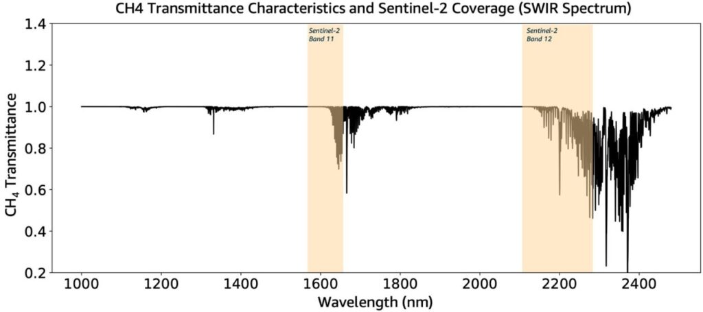
Satellite tv for pc-based methane sensing approaches usually depend on the distinctive transmittance traits of CH4. Within the seen spectrum, CH4 has transmittance values equal or near 1, that means it’s undetectable by the bare eye. Throughout sure wavelengths, nonetheless, methane does soak up mild (transmittance <1), a property which may be exploited for detection functions. For this, the quick wavelength infrared (SWIR) spectrum (1500–2500 nm spectral vary) is usually chosen, which is the place CH4 is most detectable. Hyper- and multispectral satellite tv for pc missions (that’s, these with optical devices that seize picture knowledge inside a number of wavelength ranges (bands) throughout the electromagnetic spectrum) cowl these SWIR ranges and subsequently characterize potential detection devices. Determine 1 plots the transmittance traits of methane within the SWIR spectrum and the SWIR protection of assorted candidate multispectral satellite tv for pc devices (tailored from this examine).

Determine 1 – Transmittance traits of methane within the SWIR spectrum and protection of Sentinel-2 multi-spectral missions
Many multispectral satellite tv for pc missions are restricted both by a low revisit frequency (for instance, PRISMA Hyperspectral at roughly 16 days) or by low spatial decision (for instance, Sentinel 5 at 7.5 km x 7.5 km). The price of accessing knowledge is an extra problem: some devoted constellations function as industrial missions, doubtlessly making CH4 emission insights much less available to researchers, choice makers, and different involved events because of monetary constraints. ESA’s Sentinel-2 multispectral mission, which this answer relies on, strikes an applicable steadiness between revisit fee (roughly 5 days), spatial decision (roughly 20 m) and open entry (hosted on the AWS Registry of Open Data).
Sentinel-2 has two bands that cover the SWIR spectrum (at a 20 m decision): band-11 (1610 nm central wavelength) and band-12 (2190 nm central wavelength). Each bands are appropriate for methane detection, whereas band-12 has considerably increased sensitivity to CH4 absorption (see Determine 1). Intuitively there are two potential approaches to utilizing this SWIR reflectance knowledge for methane detection. First, you possibly can give attention to only a single SWIR band (ideally the one that’s most delicate to CH4 absorption) and compute the pixel-by-pixel distinction in reflectance throughout two completely different satellite tv for pc passes. Alternatively, you employ knowledge from a single satellite tv for pc go for detection by utilizing the 2 adjoining spectral SWIR bands which have related floor and aerosol reflectance properties however have completely different methane absorption traits.
The detection technique we implement on this weblog put up combines each approaches. We draw on recent findings from the earth observation literature and compute the fractional change in top-of-the-atmosphere (TOA) reflectance Δρ (that’s, reflectance measured by Sentinel-2 together with contributions from atmospheric aerosols and gases) between two satellite tv for pc passes and the 2 SWIR bands; one baseline go the place no methane is current (base) and one monitoring go the place an lively methane level supply is suspected (monitor). Mathematically, this may be expressed as follows:
 Equation (1)
the place ρ is the TOA reflectance as measured by Sentinel-2, cmonitor and cbase are computed by regressing TOA reflectance values of band-12 towards these of band-11 throughout all the scene (that’s, ρb11 = c * ρb12). For extra particulars, consult with this examine on high-frequency monitoring of anomalous methane point sources with multispectral Sentinel-2 satellite observations.
Implement a methane detection algorithm with SageMaker geospatial capabilities
To implement the methane detection algorithm, we use the SageMaker geospatial pocket book inside Amazon SageMaker Studio. The geospatial pocket book kernel is pre-equipped with important geospatial libraries resembling GDAL, GeoPandas, Shapely, xarray, and Rasterio, enabling direct visualization and processing of geospatial knowledge inside the Python pocket book setting. See the getting started guide to learn to begin utilizing SageMaker geospatial capabilities.
SageMaker supplies a purpose-built API designed to facilitate the retrieval of satellite tv for pc imagery by a consolidated interface utilizing the SearchRasterDataCollection API name. SearchRasterDataCollection depends on the next enter parameters:
Arn: The Amazon useful resource identify (ARN) of the queried raster knowledge assortmentAreaOfInterest: A polygon object (in GeoJSON format) representing the area of curiosity for the search questionTimeRangeFilter: Defines the time vary of curiosity, denoted as{StartTime: <string>,EndTime: <string>}PropertyFilters: Supplementary property filters, resembling specs for max acceptable cloud cowl, may also be integrated
This technique helps querying from numerous raster knowledge sources which may be explored by calling ListRasterDataCollections. Our methane detection implementation makes use of Sentinel-2 satellite imagery, which may be globally referenced utilizing the next ARN: arn:aws:sagemaker-geospatial:us-west-2:378778860802:raster-data-collection/public/nmqj48dcu3g7ayw8.
This ARN represents Sentinel-2 imagery, which has been processed to Degree 2A (floor reflectance, atmospherically corrected). For methane detection functions, we are going to use top-of-atmosphere (TOA) reflectance knowledge (Degree 1C), which doesn’t embody the floor degree atmospheric corrections that might make adjustments in aerosol composition and density (that’s, methane leaks) undetectable.
To determine potential emissions from a particular level supply, we want two enter parameters: the coordinates of the suspected level supply and a chosen timestamp for methane emission monitoring. On condition that the SearchRasterDataCollection API makes use of polygons or multi-polygons to outline an space of curiosity (AOI), our strategy includes increasing the purpose coordinates right into a bounding field first after which utilizing that polygon to question for Sentinel-2 imagery utilizing SearchRasterDateCollection.
On this instance, we monitor a identified methane leak originating from an oil area in Northern Africa. It is a commonplace validation case within the distant sensing literature and is referenced, for instance, in this examine. A totally executable code base is offered on the amazon-sagemaker-examples GitHub repository. Right here, we spotlight solely chosen code sections that characterize the important thing constructing blocks for implementing a methane detection answer with SageMaker geospatial capabilities. See the repository for added particulars.
We begin by initializing the coordinates and goal monitoring date for the instance case.
#coordinates and date for North Africa oil area
#see right here for reference: https://doi.org/10.5194/amt-14-2771-2021
point_longitude = 5.9053
point_latitude = 31.6585
target_date="2019-11-20"
#measurement of bounding field in every route round level
distance_offset_meters = 1500
The next code snippet generates a bounding field for the given level coordinates after which performs a seek for the accessible Sentinel-2 imagery primarily based on the bounding field and the desired monitoring date:
def bbox_around_point(lon, lat, distance_offset_meters):
    #Equatorial radius (km) taken from https://nssdc.gsfc.nasa.gov/planetary/factsheet/earthfact.html
    earth_radius_meters = 6378137
    lat_offset = math.levels(distance_offset_meters / earth_radius_meters)
    lon_offset = math.levels(distance_offset_meters / (earth_radius_meters * math.cos(math.radians(lat))))
    return geometry.Polygon([
        [lon - lon_offset, lat - lat_offset],
        [lon - lon_offset, lat + lat_offset],
        [lon + lon_offset, lat + lat_offset],
        [lon + lon_offset, lat - lat_offset],
        [lon - lon_offset, lat - lat_offset],
    ])

#generate bounding field and extract polygon coordinates
aoi_geometry = bbox_around_point(point_longitude, point_latitude, distance_offset_meters)
aoi_polygon_coordinates = geometry.mapping(aoi_geometry)['coordinates']

#set search parameters
search_params = {
    "Arn": "arn:aws:sagemaker-geospatial:us-west-2:378778860802:raster-data-collection/public/nmqj48dcu3g7ayw8", # Sentinel-2 L2 knowledge
    "RasterDataCollectionQuery": {
        "AreaOfInterest": {
            "AreaOfInterestGeometry": {
                "PolygonGeometry": {
                    "Coordinates": aoi_polygon_coordinates
                }
            }
        },
        "TimeRangeFilter": {
            "StartTime": "{}T00:00:00Z".format(as_iso_date(target_date)),
            "EndTime": "{}T23:59:59Z".format(as_iso_date(target_date))
        }
    },
}
#question raster knowledge utilizing SageMaker geospatial capabilities
sentinel2_items = geospatial_client.search_raster_data_collection(**search_params)
The response incorporates a listing of matching Sentinel-2 gadgets and their corresponding metadata. These embody Cloud-Optimized GeoTIFFs (COG) for all Sentinel-2 bands, in addition to thumbnail photos for a fast preview of the visible bands of the picture. Naturally, it’s additionally potential to entry the full-resolution satellite tv for pc picture (RGB plot), proven in Determine 2 that follows.
 Determine 2 – Satellite tv for pc picture (RGB plot) of AOI
As beforehand detailed, our detection strategy depends on fractional adjustments in top-of-the-atmosphere (TOA) SWIR reflectance. For this to work, the identification of an excellent baseline is essential. Discovering an excellent baseline can shortly turn out to be a tedious course of that includes loads of trial and error. Nonetheless, good heuristics can go a good distance in automating this search course of. A search heuristic that has labored nicely for instances investigated up to now is as follows: for the previous day_offset=n days, retrieve all satellite tv for pc imagery, take away any clouds and clip the picture to the AOI in scope. Then compute the common band-12 reflectance throughout the AOI. Return the Sentinel tile ID of the picture with the very best common reflectance in band-12.
This logic is carried out within the following code excerpt. Its rationale depends on the truth that band-12 is very delicate to CH4 absorption (see Determine 1). A higher common reflectance worth corresponds to a decrease absorption from sources resembling methane emissions and subsequently supplies a robust indication for an emission free baseline scene.
def approximate_best_reference_date(lon, lat, date_to_monitor, distance_offset=1500, cloud_mask=True, day_offset=30):

    #initialize AOI and different parameters
    aoi_geometry = bbox_around_point(lon, lat, distance_offset)
    BAND_12_SWIR22 = "B12"
    max_mean_swir = None
    ref_s2_tile_id = None
    ref_target_date = date_to_monitor

    #loop over n=day_offset earlier days
    for day_delta in vary(-1 * day_offset, 0):
        date_time_obj = datetime.strptime(date_to_monitor, '%Y-%m-%d')
        target_date = (date_time_obj + timedelta(days=day_delta)).strftime('%Y-%m-%d')

        #get Sentinel-2 tiles for present date
        s2_tiles_for_target_date = get_sentinel2_meta_data(target_date, aoi_geometry)

        #loop over accessible tiles for present date
        for s2_tile_meta in s2_tiles_for_target_date:
            s2_tile_id_to_test = s2_tile_meta['Id']
            #retrieve cloud-masked (optionally available) L1C band 12
            target_band_data = get_s2l1c_band_data_xarray(s2_tile_id_to_test, BAND_12_SWIR22, clip_geometry=aoi_geometry, cloud_mask=cloud_mask)
            #compute imply reflectance of SWIR band
            mean_swir = target_band_data.sum() / target_band_data.depend()

            #make sure the seen/non-clouded space is sufficiently massive
            visible_area_ratio = target_band_data.depend() / (target_band_data.form[1] * target_band_data.form[2])
            if visible_area_ratio <= 0.7: #<-- guarantee acceptable cloud cowl
                proceed

            #replace most ref_s2_tile_id and ref_target_date if relevant
            if max_mean_swir is None or mean_swir > max_mean_swir:
                max_mean_swir = mean_swir
                ref_s2_tile_id = s2_tile_id_to_test
                ref_target_date = target_date

    return (ref_s2_tile_id, ref_target_date)
Utilizing this technique permits us to approximate an appropriate baseline date and corresponding Sentinel-2 tile ID. Sentinel-2 tile IDs carry info on the mission ID (Sentinel-2A/Sentinel-2B), the distinctive tile quantity (resembling, 32SKA), and the date the picture was taken amongst different info and uniquely determine an remark (that’s, a scene). In our instance, the approximation course of suggests October 6, 2019 (Sentinel-2 tile: S2B_32SKA_20191006_0_L2A), as probably the most appropriate baseline candidate.
Subsequent, we are able to compute the corrected fractional change in reflectance between the baseline date and the date we’d like to observe. The correction elements c (see Equation 1 previous) may be calculated with the next code:
def compute_correction_factor(tif_y, tif_x):

    #get flattened arrays for regression
    y = np.array(tif_y.values.flatten())
    x = np.array(tif_x.values.flatten())
    np.nan_to_num(y, copy=False)
    np.nan_to_num(x, copy=False)

    #match linear mannequin utilizing least squares regression
    x = x[:,np.newaxis] #reshape
    c, _, _, _ = np.linalg.lstsq(x, y, rcond=None)

    return c[0]
The total implementation of Equation 1 is given within the following code snippet:
def compute_corrected_fractional_reflectance_change(l1_b11_base, l1_b12_base, l1_b11_monitor, l1_b12_monitor):

    #get correction elements
    c_monitor = compute_correction_factor(tif_y=l1_b11_monitor, tif_x=l1_b12_monitor)
    c_base = compute_correction_factor(tif_y=l1_b11_base, tif_x=l1_b12_base)

    #get corrected fractional reflectance change
    frac_change = ((c_monitor*l1_b12_monitor-l1_b11_monitor)/l1_b11_monitor)-((c_base*l1_b12_base-l1_b11_base)/l1_b11_base)
    return frac_change
Lastly, we are able to wrap the above strategies into an end-to-end routine that identifies the AOI for a given longitude and latitude, monitoring date and baseline tile, acquires the required satellite tv for pc imagery, and performs the fractional reflectance change computation.
def run_full_fractional_reflectance_change_routine(lon, lat, date_monitor, baseline_s2_tile_id, distance_offset=1500, cloud_mask=True):

    #get bounding field
    aoi_geometry = bbox_around_point(lon, lat, distance_offset)

    #get S2 metadata
    s2_meta_monitor = get_sentinel2_meta_data(date_monitor, aoi_geometry)

    #get tile id
    grid_id = baseline_s2_tile_id.break up("_")[1]
    s2_tile_id_monitor = record(filter(lambda x: f"_{grid_id}_" in x["Id"], s2_meta_monitor))[0]["Id"]

    #retrieve band 11 and 12 of the Sentinel L1C product for the given S2 tiles
    l1_swir16_b11_base = get_s2l1c_band_data_xarray(baseline_s2_tile_id, BAND_11_SWIR16, clip_geometry=aoi_geometry, cloud_mask=cloud_mask)
    l1_swir22_b12_base = get_s2l1c_band_data_xarray(baseline_s2_tile_id, BAND_12_SWIR22, clip_geometry=aoi_geometry, cloud_mask=cloud_mask)
    l1_swir16_b11_monitor = get_s2l1c_band_data_xarray(s2_tile_id_monitor, BAND_11_SWIR16, clip_geometry=aoi_geometry, cloud_mask=cloud_mask)
    l1_swir22_b12_monitor = get_s2l1c_band_data_xarray(s2_tile_id_monitor, BAND_12_SWIR22, clip_geometry=aoi_geometry, cloud_mask=cloud_mask)

    #compute corrected fractional reflectance change
    frac_change = compute_corrected_fractional_reflectance_change(
        l1_swir16_b11_base,
        l1_swir22_b12_base,
        l1_swir16_b11_monitor,
        l1_swir22_b12_monitor
    )

    return frac_change
Working this technique with the parameters we decided earlier yields the fractional change in SWIR TOA reflectance as an xarray.DataArray. We are able to carry out a primary visible inspection of the consequence by operating a easy plot() invocation on this knowledge array. Our technique reveals the presence of a methane plume on the middle of the AOI that was undetectable within the RGB plot seen beforehand.
 Determine 3 – Fractional reflectance change in TOA reflectance (SWIR spectrum)
As a ultimate step, we extract the recognized methane plume and overlay it on a uncooked RGB satellite tv for pc picture to offer the vital geographic context. That is achieved by thresholding, which may be carried out as proven within the following:
def get_plume_mask(change_in_reflectance_tif, threshold_value):
    cr_masked = change_in_reflectance_tif.copy()
    #set values above threshold to nan
    cr_masked[cr_masked > treshold_value] = np.nan
    #apply masks on nan values
    plume_tif = np.ma.array(cr_masked, masks=cr_masked==np.nan)

    return plume_tif
For our case, a threshold of -0.02 fractional change in reflectance yields good outcomes however this could change from scene to scene and you’ll have to calibrate this to your particular use case. Determine 4 that follows illustrates how the plume overlay is generated by combining the uncooked satellite tv for pc picture of the AOI with the masked plume right into a single composite picture that exhibits the methane plume in its geographic context.

Determine 4 – RGB picture, fractional reflectance change in TOA reflectance (SWIR spectrum), and methane plume overlay for AOI
Resolution validation with real-world methane emission occasions
As a ultimate step, we consider our technique for its skill to appropriately detect and pinpoint methane leakages from a spread of sources and geographies. First, we use a managed methane launch experiment particularly designed for the validation of space-based point-source detection and quantification of onshore methane emissions. On this 2021 experiment, researchers carried out a number of methane releases in Ehrenberg, Arizona over a 19-day interval. Working our detection technique for one of many Sentinel-2 passes in the course of the time of that experiment produces the next consequence exhibiting a methane plume:
 Determine 5 – Methane plume intensities for Arizona Managed Launch Experiment
The plume generated in the course of the managed launch is clearly recognized by our detection technique. The identical is true for different identified real-world leakages (in Determine 6 that follows) from sources resembling a landfill in East Asia (left) or an oil and gasoline facility in North America (proper).
 Determine 6 – Methane plume intensities for an East Asian landfill (left) and an oil and gasoline area in North America (proper)
In sum, our technique may also help determine methane emissions each from managed releases and from numerous real-world level sources throughout the globe. This works greatest for on-shore level sources with restricted surrounding vegetation. It doesn’t work for off-shore scenes because of the high absorption (that is, low transmittance) of the SWIR spectrum by water. On condition that the proposed detection algorithm depends on variations in methane depth, our technique additionally requires pre-leakage observations. This will make monitoring of leakages with fixed emission charges difficult.
Clear up
To keep away from incurring undesirable prices after a methane monitoring job has accomplished, be sure that you terminate the SageMaker occasion and delete any undesirable native recordsdata.
Conclusion
By combining SageMaker geospatial capabilities with open geospatial knowledge sources you’ll be able to implement your individual extremely personalized distant monitoring options at scale. This weblog put up targeted on methane detection, a focal space for governments, NGOs and different organizations looking for to detect and in the end keep away from dangerous methane emissions. You will get began right now in your individual journey into geospatial analytics by spinning up a Pocket book with the SageMaker geospatial kernel and implement your individual detection answer. See the GitHub repository to get began constructing your individual satellite-based methane detection answer. Additionally take a look at the sagemaker-examples repository for additional examples and tutorials on how you can use SageMaker geospatial capabilities in different real-world distant sensing functions.
In regards to the authors
 Dr. Karsten Schroer is a Options Architect at AWS. He helps clients in leveraging knowledge and know-how to drive sustainability of their IT infrastructure and construct cloud-native data-driven options that allow sustainable operations of their respective verticals. Karsten joined AWS following his PhD research in utilized machine studying & operations administration. He’s really obsessed with technology-enabled options to societal challenges and likes to dive deep into the strategies and utility architectures that underlie these options.
 Janosch Woschitz is a Senior Options Architect at AWS, specializing in geospatial AI/ML. With over 15 years of expertise, he helps clients globally in leveraging AI and ML for modern options that capitalize on geospatial knowledge. His experience spans machine studying, knowledge engineering, and scalable distributed programs, augmented by a robust background in software program engineering and business experience in complicated domains resembling autonomous driving.