First experiments with TensorFlow mixed-precision coaching
Ranging from its – very – current 2.1 launch, TensorFlow helps what known as mixed-precision coaching (within the following: MPT) for Keras. On this submit, we experiment with MPT and supply some background. Said upfront: On a Tesla V100 GPU, our CNN-based experiment didn’t reveal substantial reductions in execution time. In a case like this, it’s laborious to determine whether or not to truly write a submit or not. You might argue that identical to in science, null outcomes are outcomes. Or, extra virtually: They open up a dialogue which will result in bug discovery, clarification of utilization directions, and additional experimentation, amongst others.
As well as, the subject itself is fascinating sufficient to deserve some background explanations – even when the outcomes usually are not fairly there but.
So to begin, let’s hear some context on MPT.
This isn’t nearly saving reminiscence
One technique to describe MPT in TensorFlow may go like this: MPT permits you to practice fashions the place the weights are of sort float32 or float64, as typical (for causes of numeric stability), however the knowledge – the tensors pushed between operations – have decrease precision, particularly, 16bit (float16).
This sentence would in all probability do nice as a TLDR;
for the new-ish MPT documentation page, additionally out there for R on the TensorFlow for R website. And primarily based on this sentence, you is likely to be result in suppose “oh positive, so that is about saving reminiscence”. Much less reminiscence utilization would then suggest you would run bigger batch sizes with out getting out-of-memory errors.
That is after all right, and also you’ll see it occurring within the experimentation outcomes.
Nevertheless it’s solely a part of the story. The opposite half is expounded to GPU structure and parallel (not simply parallel on-GPU, as we’ll see) computing.
AVX & co.
GPUs are all about parallelization. However for CPUs as effectively, the final ten years have seen essential developments in structure and instruction units. SIMD (Single Instruction Multiple Data) operations carry out one instruction over a bunch of information directly. For instance, two 128-bit operands may maintain two 64-bit integers every, and these could possibly be added pairwise. Conceptually, this reminds of vector addition in R (it’s simply an analogue although!):
Or, these operands may comprise 4 32-bit integers every, wherein case we may symbolically write
With 16-bit integers, we may once more double the variety of parts operated upon:
During the last decade, the foremost SIMD-related X-86 meeting language extensions have been AVX (Superior Vector Extensions), AVX2, AVX-512, and FMA (extra on FMA quickly).
Do any of those ring a bell?
Your CPU helps directions that this TensorFlow binary was not compiled to make use of:
AVX2 FMA
It is a line you might be prone to see if you’re utilizing a pre-built TensorFlow binary, versus compiling from supply. (Later, when reporting experimentation outcomes, we may also point out on-CPU execution occasions, to supply some context for the GPU execution occasions we’re fascinated with – and only for enjoyable, we’ll additionally do a – very superficial – comparability between a TensorFlow binary put in from PyPi and one which was compiled manually.)
Whereas all these AVXes are (mainly) about an extension of vector processing to bigger and bigger knowledge varieties, FMA is totally different, and it’s an fascinating factor to find out about in itself – for anybody doing sign processing or utilizing neural networks.
Fused Multiply-Add (FMA)
Fused Multiply-Add is a sort of multiply-accumulate operation. In multiply-accumulate, operands are multiplied after which added to accumulator protecting monitor of the operating sum. If “fused”, the entire multiply-then-add operation is carried out with a single rounding on the finish (versus rounding as soon as after the multiplication, after which once more after the addition). Often, this ends in greater accuracy.
For CPUs, FMA was launched concurrently with AVX2. FMA could be carried out on scalars or on vectors, “packed” in the best way described within the earlier paragraph.
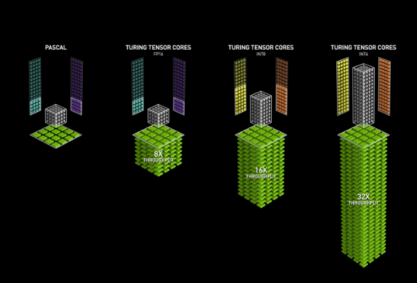
Why did we are saying this was so fascinating to knowledge scientists? Nicely, a whole lot of operations – dot merchandise, matrix multiplications, convolutions – contain multiplications adopted by additions. “Matrix multiplication” right here really has us depart the realm of CPUs and leap to GPUs as a substitute, as a result of what MPT does is make use of the new-ish NVidia Tensor Cores that reach FMA from scalars/vectors to matrices.
Tensor Cores
As documented, MPT requires GPUs with compute capability >= 7.0. The respective GPUs, along with the same old Cuda Cores, have so referred to as “Tensor Cores” that carry out FMA on matrices:
The operation takes place on 4×4 matrices; multiplications occur on 16-bit operands whereas the ultimate end result could possibly be 16-bit or 32-bit.
We will see how that is instantly related to the operations concerned in deep studying; the small print, nonetheless, are not necessarily clear.
Leaving these internals to the specialists, we now proceed to the precise experiment.
Experiments
Dataset
With their 28x28px / 32x32px sized photographs, neither MNIST nor CIFAR appeared notably suited to problem the GPU. As a substitute, we selected Imagenette, the “little ImageNet” created by the quick.ai people, consisting of 10 lessons: tench, English springer, cassette participant, chain noticed, church, French horn, rubbish truck, fuel pump, golf ball, and parachute. Listed here are a couple of examples, taken from the 320px model:

Determine 3: Examples of the ten lessons of Imagenette.
These photographs have been resized – protecting the facet ratio – such that the bigger dimension has size 320px. As a part of preprocessing, we’ll additional resize to 256x256px, to work with a pleasant energy of two.
The dataset could conveniently be obtained through utilizing tfds, the R interface to TensorFlow Datasets.
library(keras)
# wants model 2.1
library(tensorflow)
library(tfdatasets)
# out there from github: devtools::install_github("rstudio/tfds")
library(tfds)

# to make use of TensorFlow Datasets, we'd like the Python backend
# usually, simply use tfds::install_tfds for this
# as of this writing although, we'd like a nightly construct of TensorFlow Datasets
# envname ought to check with no matter setting you run TensorFlow in
reticulate::py_install("tfds-nightly", envname = "r-reticulate")

# on first execution, this downloads the dataset
imagenette <- tfds_load("imagenette/320px")

# extract practice and check components
practice <- imagenette$practice
check <- imagenette$validation

# batch dimension for the preliminary run
batch_size <- 32
# 12895 is the variety of objects within the coaching set
buffer_size <- 12895/batch_size

# coaching dataset is resized, scaled to between 0 and 1,
# cached, shuffled, and divided into batches
train_dataset <- practice %>%
  dataset_map(operate(document) {
    document$picture <- document$picture %>%
      tf$picture$resize(dimension = c(256L, 256L)) %>%
      tf$truediv(255)
    document
  }) %>%
  dataset_cache() %>%
  dataset_shuffle(buffer_size) %>%
  dataset_batch(batch_size) %>%
  dataset_map(unname)

# check dataset is resized, scaled to between 0 and 1, and divided into batches
test_dataset <- check %>%
  dataset_map(operate(document) {
    document$picture <- document$picture %>%
      tf$picture$resize(dimension = c(256L, 256L)) %>%
      tf$truediv(255)
    document}) %>%
  dataset_batch(batch_size) %>%
  dataset_map(unname)
Within the above code, we cache the dataset after the resize and scale operations, as we need to reduce preprocessing time spent on the CPU.
Configuring MPT
Our experiment makes use of Keras match – versus a customized coaching loop –, and given these preconditions, operating MPT is usually a matter of including three traces of code. (There’s a small change to the mannequin, as we’ll see in a second.)
We inform Keras to make use of the mixed_float16 Coverage, and confirm that the tensors have sort float16 whereas the Variables (weights) nonetheless are of sort float32:
# should you learn this at a later time and get an error right here,
# try whether or not the situation within the codebase has modified
mixed_precision <- tf$keras$mixed_precision$experimental

coverage <- mixed_precision$Coverage('mixed_float16')
mixed_precision$set_policy(coverage)

# float16
coverage$compute_dtype
# float32
coverage$variable_dtype
The mannequin is an easy convnet, with numbers of filters being multiples of 8, as specified within the documentation. There’s one factor to notice although: For causes of numerical stability, the precise output tensor of the mannequin needs to be of sort float32.
mannequin <- keras_model_sequential() %>%
  layer_conv_2d(filters = 32, kernel_size = 5, strides = 2, padding = "identical", input_shape = c(256, 256, 3), activation = "relu") %>%
  layer_batch_normalization() %>%
  layer_conv_2d(filters = 64, kernel_size = 7, strides = 2, padding = "identical", activation = "relu") %>%
  layer_batch_normalization() %>%
  layer_conv_2d(filters = 128, kernel_size = 11, strides = 2, padding = "identical", activation = "relu") %>%
  layer_batch_normalization() %>%
  layer_global_average_pooling_2d() %>%
  # separate logits from activations so precise outputs could be float32
  layer_dense(items = 10) %>%
  layer_activation("softmax", dtype = "float32")

mannequin %>% compile(
  loss = "sparse_categorical_crossentropy",
  optimizer = "adam",
  metrics = "accuracy")

mannequin %>%
  match(train_dataset, validation_data = test_dataset, epochs = 20)
Outcomes
The principle experiment was executed on a Tesla V100 with 16G of reminiscence. Only for curiosity, we ran that very same mannequin below 4 different situations, none of which fulfill the prerequisite of getting a compute functionality equal to at the least 7.0. We’ll rapidly point out these after the principle outcomes.
With the above mannequin, closing accuracy (closing as in: after 20 epochs) fluctuated about 0.78:
Epoch 16/20
403/403 [==============================] - 12s 29ms/step - loss: 0.3365 -
accuracy: 0.8982 - val_loss: 0.7325 - val_accuracy: 0.8060
Epoch 17/20
403/403 [==============================] - 12s 29ms/step - loss: 0.3051 -
accuracy: 0.9084 - val_loss: 0.6683 - val_accuracy: 0.7820
Epoch 18/20
403/403 [==============================] - 11s 28ms/step - loss: 0.2693 -
accuracy: 0.9208 - val_loss: 0.8588 - val_accuracy: 0.7840
Epoch 19/20
403/403 [==============================] - 11s 28ms/step - loss: 0.2274 -
accuracy: 0.9358 - val_loss: 0.8692 - val_accuracy: 0.7700
Epoch 20/20
403/403 [==============================] - 11s 28ms/step - loss: 0.2082 -
accuracy: 0.9410 - val_loss: 0.8473 - val_accuracy: 0.7460
The numbers reported beneath are milliseconds per step, step being a move over a single batch. Thus usually, doubling the batch dimension we might anticipate execution time to double as effectively.
Listed here are execution occasions, taken from epoch 20, for 5 totally different batch sizes, evaluating MPT with a default Coverage that makes use of float32 all through. (We must always add that aside from the very first epoch, execution occasions per step fluctuated by at most one millisecond in each situation.)
| 32 | 28 | 30 |
| 64 | 52 | 56 |
| 128 | 97 | 106 |
| 256 | 188 | 206 |
| 512 | 377 | 415 |
Constantly, MPT was sooner, indicating that the meant code path was used.
However the speedup just isn’t that massive.
We additionally watched GPU utilization in the course of the runs. These ranged from round 72% for batch_size 32 over ~ 78% for batch_size 128 to hightly fluctuating values, repeatedly reaching 100%, for batch_size 512.
As alluded to above, simply to anchor these values we ran the identical mannequin in 4 different situations, the place no speedup was to be anticipated. Despite the fact that these execution occasions usually are not strictly a part of the experiments, we report them, in case the reader is as interested by some context as we have been.
Firstly, right here is the equal desk for a Titan XP with 12G of reminiscence and compute functionality 6.1.
| 32 | 44 | 38 |
| 64 | 70 | 70 |
| 128 | 142 | 136 |
| 256 | 270 | 270 |
| 512 | 518 | 539 |
As anticipated, there isn’t any constant superiority of MPT; as an apart, wanting on the values total (particularly as in comparison with CPU execution occasions to come back!) you may conclude that fortunately, one doesn’t at all times want the most recent and best GPU to coach neural networks!
Subsequent, we take one additional step down the {hardware} ladder. Listed here are execution occasions from a Quadro M2200 (4G, compute functionality 5.2). (The three runs that don’t have a quantity crashed with out of reminiscence.)
| 32 | 186 | 197 |
| 64 | 352 | 375 |
| 128 | 687 | 746 |
| 256 | 1000 | – |
| 512 | – | – |
This time, we really see how the pure memory-usage facet performs a job: With MPT, we will run batches of dimension 256; with out, we get an out-of-memory error.
Now, we additionally in contrast with runtime on CPU (Intel Core I7, clock pace 2.9Ghz). To be sincere, we stopped after a single epoch although. With a batch_size of 32 and operating a normal pre-built set up of TensorFlow, a single step now took 321 – not milliseconds, however seconds. Only for enjoyable, we in comparison with a manually constructed TensorFlow that may make use of AVX2 and FMA directions (this matter may actually deserve a devoted experiment): Execution time per step was diminished to 304 seconds/step.
Conclusion
Summing up, our experiment didn’t present essential reductions in execution occasions – for causes as but unclear. We’d be completely satisfied to encourage a dialogue within the feedback!
Experimental outcomes however, we hope you’ve loved getting some background data on a not-too-frequently mentioned matter. Thanks for studying!