Utilizing Amazon SageMaker with Level Clouds: Half 1- Floor Fact for 3D labeling

On this two-part sequence, we display easy methods to label and prepare fashions for 3D object detection duties. Partially 1, we talk about the dataset we’re utilizing, in addition to any preprocessing steps, to know and label knowledge. Partially 2, we stroll via easy methods to prepare a mannequin in your dataset and deploy it to manufacturing.

LiDAR (gentle detection and ranging) is a technique for figuring out ranges by focusing on an object or floor with a laser and measuring the time for the mirrored gentle to return to the receiver. Autonomous automobile corporations sometimes use LiDAR sensors to generate a 3D understanding of the surroundings round their automobiles.

As LiDAR sensors turn out to be extra accessible and cost-effective, clients are more and more utilizing level cloud knowledge in new areas like robotics, sign mapping, and augmented actuality. Some new cellular units even embody LiDAR sensors. The rising availability of LiDAR sensors has elevated curiosity in level cloud knowledge for machine studying (ML) duties, like 3D object detection and monitoring, 3D segmentation, 3D object synthesis and reconstruction, and utilizing 3D knowledge to validate 2D depth estimation.

On this sequence, we present you easy methods to prepare an object detection mannequin that runs on level cloud knowledge to foretell the situation of automobiles in a 3D scene. This put up, we focus particularly on labeling LiDAR knowledge. Commonplace LiDAR sensor output is a sequence of 3D level cloud frames, with a typical seize fee of 10 frames per second. To label this sensor output you want a labeling software that may deal with 3D knowledge. Amazon SageMaker Ground Truth makes it straightforward to label objects in a single 3D body or throughout a sequence of 3D level cloud frames for constructing ML coaching datasets. Floor Fact additionally helps sensor fusion of digital camera and LiDAR knowledge with as much as eight video digital camera inputs.

Knowledge is crucial to any ML venture. 3D knowledge specifically will be tough to supply, visualize, and label. We use the A2D2 dataset on this put up and stroll you thru the steps to visualise and label it.

A2D2 accommodates 40,000 frames with semantic segmentation and level cloud labels, together with 12,499 frames with 3D bounding field labels. Since we’re specializing in object detection, we’re within the 12,499 frames with 3D bounding field labels. These annotations embody 14 courses related to driving like automotive, pedestrian, truck, bus, and so forth.

The next desk reveals the whole class record:

We are going to prepare our detector to particularly detect automobiles since that’s the commonest class in our dataset (32616 of the 42816 whole objects within the dataset are labeled as automobiles).

Answer overview

On this sequence, we cowl easy methods to visualize and label your knowledge with Amazon SageMaker Floor Fact and display easy methods to use this knowledge in an Amazon SageMaker coaching job to create an object detection mannequin, deployed to an Amazon SageMaker Endpoint. Particularly, we’ll use an Amazon SageMaker pocket book to function the answer and launch any labeling or coaching jobs.

The next diagram depicts the general circulate of sensor knowledge from labeling to coaching to deployment:

You’ll discover ways to prepare and deploy a real-time 3D object detection mannequin with Amazon SageMaker Floor Fact with the next steps:

1. Obtain and visualize a degree cloud dataset
2. Prep knowledge to be labeled with the Amazon SageMaker Ground Truth point cloud tool
3. Launch a distributed Amazon SageMaker Floor Fact coaching job with MMDetection3D
4. Consider your coaching job outcomes and profiling your useful resource utilization with Amazon SageMaker Debugger
5. Deploy an asynchronous SageMaker endpoint
6. Name the endpoint and visualizing 3D object predictions

AWS providers used to Implement this resolution

Conditions

The next diagram demonstrates easy methods to create a non-public workforce. For written, step-by-step directions, see Create an Amazon Cognito Workforce Using the Labeling Workforces Page.

Launching the AWS CloudFormation stack

Now that you simply’ve seen the construction of the answer, you deploy it into your account so you’ll be able to run an instance workflow. All of the deployment steps associated to the labeling pipeline are managed by AWS CloudFormation. This implies AWS Cloudformation creates your pocket book occasion in addition to any roles or Amazon S3 Buckets to assist operating the answer.

You’ll be able to launch the stack in AWS Area us-east-1 on the AWS CloudFormation console utilizing the Launch Stack
button. To launch the stack in a unique Area, use the directions discovered within the README of the GitHub repository.

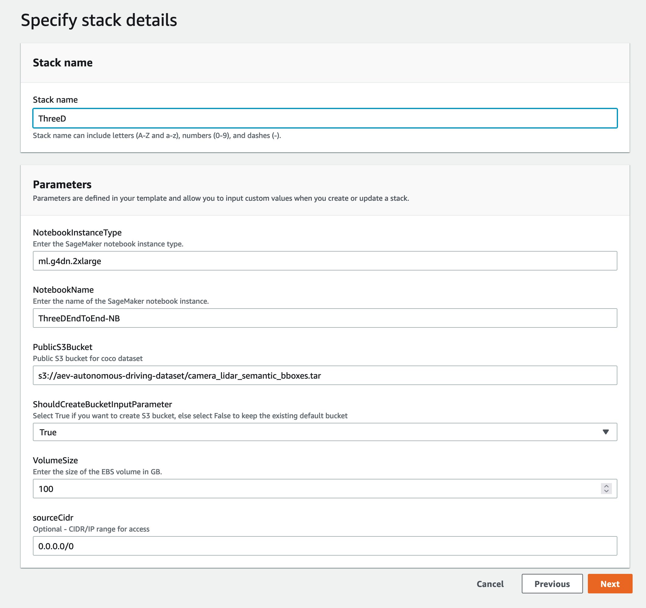
This takes roughly 20 minutes to create all of the assets. You’ll be able to monitor the progress from the AWS CloudFormation consumer interface (UI).

As soon as your CloudFormation template is finished operating return to the AWS Console.

Opening the Pocket book

Amazon SageMaker Pocket book Cases are ML compute cases that run on the Jupyter Pocket book App. Amazon SageMaker manages the creation of cases and associated assets. Use Jupyter notebooks in your pocket book occasion to arrange and course of knowledge, write code to coach fashions, deploy fashions to Amazon SageMaker internet hosting, and check or validate your fashions.

Comply with the following steps to entry the Amazon SageMaker Pocket book surroundings:

1. Underneath providers seek for Amazon SageMaker.
   
2. Underneath Pocket book, choose Pocket book cases.
   
3. A Pocket book occasion must be provisioned. Choose Open JupyterLab, which is positioned on the correct facet of the pre-provisioned Pocket book occasion below Actions.
   
4. You’ll see an icon like this because the web page hundreds:
   
5. You’ll be redirected to a brand new browser tab that appears like the next diagram:
   
6. As soon as you’re within the Amazon SageMaker Pocket book Occasion Launcher UI. From the left sidebar, choose the Git icon as proven within the following diagram.
   
7. Choose Clone a Repository choice.
   
8. Enter GitHub URL(https://github.com/aws-samples/end-2-end-3d-ml) within the pop‑up window and select clone.
   
9. Choose File Browser to see the GitHub folder.
   
10. Open the pocket book titled 1_visualization.ipynb.

Working the Pocket book

Overview

The primary few cells of the pocket book within the part titled Downloaded Recordsdata walks via easy methods to obtain the dataset and examine the recordsdata inside it. After the cells are executed, it takes a couple of minutes for the information to complete downloading.

As soon as downloaded, you’ll be able to evaluate the file construction of A2D2, which is an inventory of scenes or drives. A scene is a brief recording of sensor knowledge from our automobile. A2D2 offers 18 of those scenes for us to coach on, that are all recognized by distinctive dates. Every scene accommodates 2D digital camera knowledge, 2D labels, 3D cuboid annotations, and 3D level clouds.

You’ll be able to view the file construction for the A2D2 dataset with the next:

├── 20180807_145028
├── 20180810_142822
│   ├── digital camera
│   │   ├── cam_front_center
│   │   │   ├── 20180807145028_lidar_frontcenter_000000091.png
│   │   │   ├── 20180807145028_lidar_frontcenter_000000091.json
│   │   │   ├── 20180807145028_lidar_frontcenter_000000380.png
│   │   │   ├── 20180807145028_lidar_frontcenter_000000380.json
│   │   │   ├── ...
│   ├── label
│   │   ├── cam_front_center
│   │   │   ├── 20180807145028_lidar_frontcenter_000000091.png
│   │   │   ├── 20180807145028_lidar_frontcenter_000000380.png
│   │   │   ├── ...
│   ├── label3D
│   │   ├── cam_front_center
│   │   │   ├── 20180807145028_lidar_frontcenter_000000091.json
│   │   │   ├── 20180807145028_lidar_frontcenter_000000380.json
│   │   │   ├── ...
│   ├── lidar
│   │   ├── cam_front_center
│   │   │   ├── 20180807145028_lidar_frontcenter_000000091.npz
│   │   │   ├── 20180807145028_lidar_frontcenter_000000380.npz
│   │   │   ├── ...

A2D2 sensor setup

The subsequent part walks via studying a few of this level cloud knowledge to verify we’re deciphering it accurately and may visualize it within the pocket book earlier than attempting to transform it right into a format prepared for knowledge labeling.

For any sort of autonomous driving setup the place we’ve 2D and 3D sensor knowledge, capturing sensor calibration knowledge is crucial. Along with the uncooked knowledge, we additionally downloaded cams_lidar.json. This file accommodates the interpretation and orientation of every sensor relative to the automobile’s coordinate body, this will also be known as the sensor’s pose, or location in area. That is essential for changing factors from a sensor’s coordinate body to the automobile’s coordinate body. In different phrases, it’s essential for visualizing the 2D and 3D sensors because the automobile drives. The automobile’s coordinate body is outlined as a static level within the middle of the automobile, with the x-axis within the route of the ahead motion of the automobile, the y-axis denoting left and proper with left being constructive, and the z-axis pointing via the roof of the automobile. Some extent (X,Y,Z) of (5,2,1) means this level is 5 meters forward of our automobile, 2 meters to the left, and 1 meter above our automobile. Having these calibrations additionally permits us to venture 3D factors onto our 2D picture, which is particularly useful for level cloud labeling duties.

To see the sensor setup on the automobile, verify the next diagram.

The purpose cloud knowledge we’re coaching on is particularly aligned with the entrance going through digital camera or cam front-center: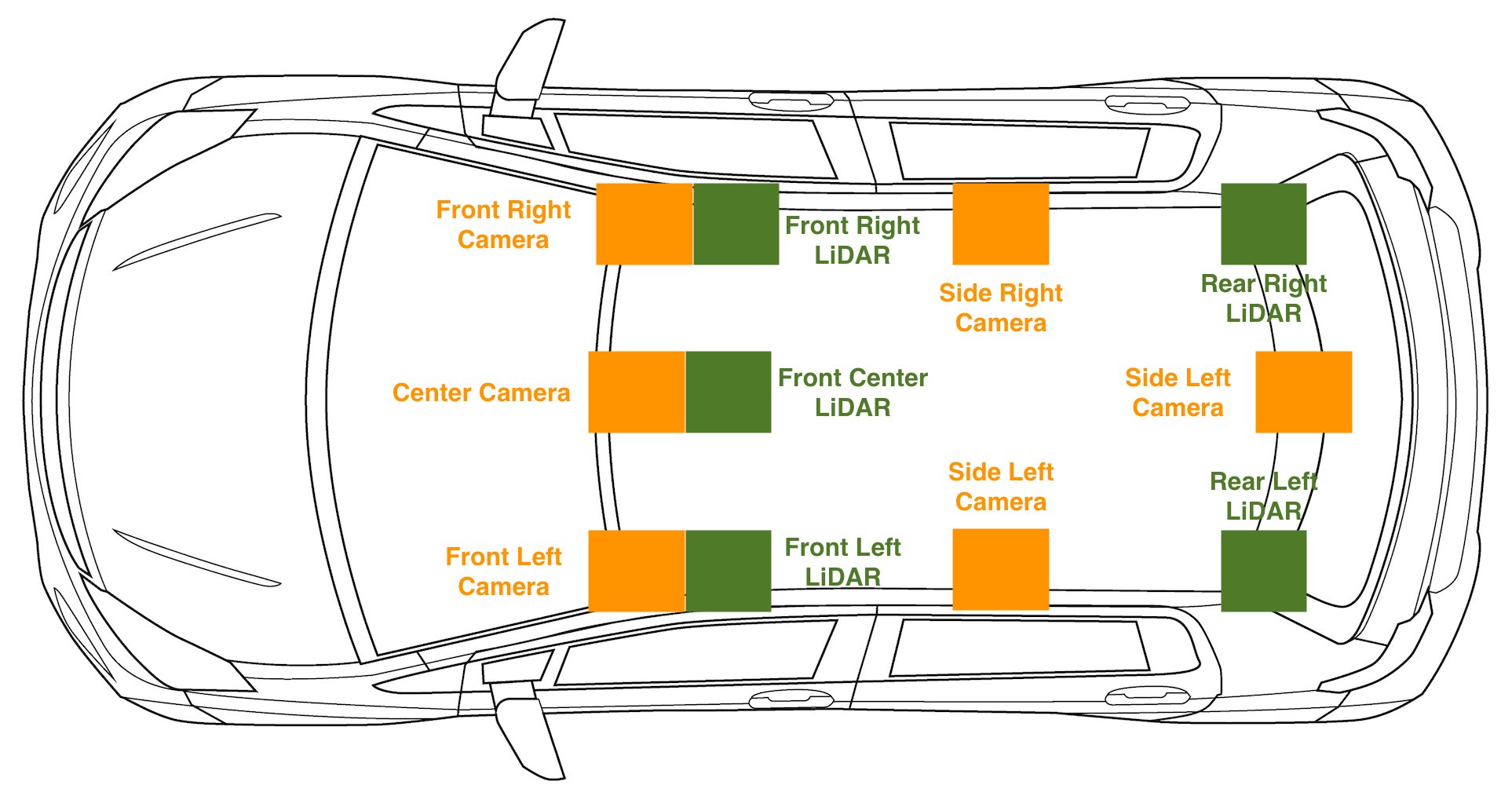

This matches our visualization of digital camera sensors in 3D:

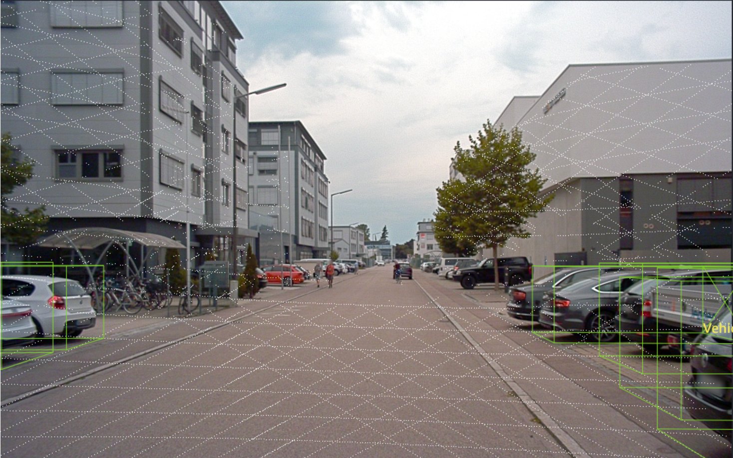
This portion of the pocket book walks via validating that the A2D2 dataset matches our expectations about sensor positions, and that we’re capable of align knowledge from the purpose cloud sensors into the digital camera body. Be happy to run all cells via the one titled Projection from 3D to 2D to see your level cloud knowledge overlay on the next digital camera picture.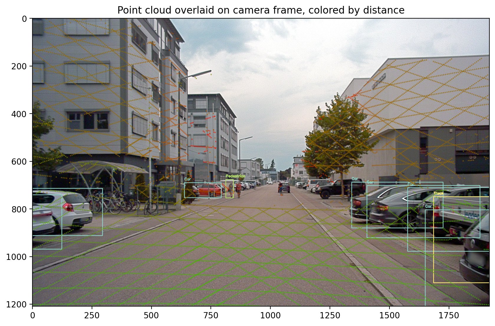

Conversion to Amazon SageMaker Floor Fact

After visualizing our knowledge in our pocket book, we will confidently convert our level clouds into Amazon SageMaker Ground Truth’s 3D format to confirm and modify our labels. This part walks via changing from A2D2’s knowledge format into an Amazon SageMaker Ground Truth sequence file, with the enter format utilized by the thing monitoring modality.

The sequence file format consists of the purpose cloud codecs, the photographs related to every level cloud, and all sensor place and orientation knowledge required to align photos with level clouds. These conversions are completed utilizing the sensor info learn from the earlier part. The next instance is a sequence file format from Amazon SageMaker Floor Fact, which describes a sequence with solely a single timestep.

The purpose cloud for this timestep is positioned at s3://sagemaker-us-east-1-322552456788/a2d2_smgt/20180807_145028_out/20180807145028_lidar_frontcenter_000000091.txt and has a format of <x coordinate> <y coordinate> <z coordinate>.

Related to the purpose cloud, is a single digital camera picture positioned at s3://sagemaker-us-east-1-322552456788/a2d2_smgt/20180807_145028_out/undistort_20180807145028_camera_frontcenter_000000091.png. Discover that we take the sequence file that defines all digital camera parameters to permit projection from the purpose cloud to the digital camera and again.

 {
 "seq-no": 1,
  "prefix": "s3://sagemaker-us-east-1-322552456788/a2d2_smgt/20180807_145028_out/",
  "number-of-frames": 1,
  "frames": [
    {
      "frame-no": 0,
      "unix-timestamp": 0.091,
      "frame": "20180807145028_lidar_frontcenter_000000091.txt",
      "format": "text/xyz",
      "ego-vehicle-pose": {
        "position": {
          "x": 0,
          "y": 0,
          "z": 0},
        "heading": {
          "qw": 1,
          "qx": 0,
          "qy": 0,
          "qz": 0}},
      "images": [
        {
          "image-path": "undistort_20180807145028_camera_frontcenter_000000091.png",
          "unix-timestamp": 0.091,
          "fx": 1687.3369140625,
          "fy": 1783.428466796875,
          "cx": 965.4341405582381,
          "cy": 684.4193604186803,
          "position": {
            "x": 1.711045726422736,
            "y": -5.735179668849011e-09,
            "z": 0.9431449279047172},
          "heading": {
            "qw": -0.4981871970275329,
            "qx": 0.5123971466375787,
            "qy": -0.4897950939891415,
            "qz": 0.4993590359047143},
          "camera-model": "pinhole"}]},
    }
  ]
}

Conversion to this enter format requires us to jot down a conversion from A2D2’s knowledge format to knowledge codecs supported by Amazon SageMaker Floor Fact. This is similar course of anybody should endure when bringing their very own knowledge for labeling. We’ll stroll via how this conversion works, step-by-step. If following alongside within the pocket book, have a look at the perform named a2d2_scene_to_smgt_sequence_and_seq_label.

Level cloud conversion

Step one is to transform the information from a compressed Numpy-formatted file (NPZ), which was generated with the numpy.savez methodology, to an accepted raw 3D format for Amazon SageMaker Floor Fact. Particularly, we generate a file with one row per level. Every 3D level is outlined by three floating level X, Y, and Z coordinates. After we specify our format within the sequence file, we use the string textual content/xyz to symbolize this format. Amazon SageMaker Floor Fact additionally helps including depth values or Purple Inexperienced Blue (RGB) factors.

A2D2’s NPZ recordsdata include a number of Numpy arrays, every with its personal title. To carry out a conversion, we load the NPZ file utilizing Numpy’s load methodology, entry the array referred to as factors (i.e., an Nx3 array, the place N is the variety of factors within the level cloud), and save as textual content to a brand new file utilizing Numpy’s savetxt methodology.

# enter.npz is an A2D2 PointCloud file
lidar_frame_contents = np.load("a2d2_input.npz")
factors = lidar_frame_contents["points"]
# output.txt is a textual content/xyz formatted SMGT file
np.savetxt("output.txt", factors)

Picture preprocessing

Subsequent, we put together our picture recordsdata. A2D2 offers PNG photos, and Amazon SageMaker Floor Fact helps PNG photos; nonetheless, these photos are distorted. Distortion usually happens as a result of the image-taking lens isn’t aligned parallel to the imaging aircraft, which makes some areas within the picture look nearer than anticipated. This distortion describes the distinction between a bodily digital camera and an idealized pinhole camera model. If distortion isn’t taken into consideration, then Amazon SageMaker Floor Fact received’t have the ability to render our 3D factors on high of the digital camera views, which makes it tougher to carry out labeling. For a tutorial on digital camera calibration, have a look at this documentation from OpenCV.

Whereas Amazon SageMaker Floor Fact helps distortion coefficients in its enter file, you may as well carry out preprocessing earlier than the labeling job. Since A2D2 offers helper code to carry out undistortion, we apply it to the picture, and go away the fields associated to distortion out of our sequence file. Notice that the distortion associated fields embody k1, k2, k3, k4, p1, p2, and skew.

from a2d2_helpers import undistort_image
# distorted_input.png comes from the A2D2 dataset
image_frame = cv2.imread("distorted_input.png")
# we undistort the front_center digital camera, and cross the cams_lidars dictionary
# which accommodates all digital camera distortion coefficients.
undistorted_image = undistort_image(image_frame, "front_center", cams_lidars)
# undistorted_output.png goes into SMGT's output path
cv2.imwrite("undistorted_output.png", undistorted_image)

Digital camera place, orientation, and projection conversion

Past the uncooked knowledge recordsdata required for labeling, the sequence file additionally requires digital camera place and orientation info to carry out the projection of 3D factors into the 2D digital camera views. We have to know the place the digital camera is trying in 3D area to determine how 3D cuboid labels and 3D factors must be rendered on high of our photos.

As a result of we’ve loaded our sensor positions into a standard rework supervisor within the A2D2 sensor setup part, we will simply question the rework supervisor for the data we would like. In our case, we deal with the automobile place as (0, 0, 0) in every body as a result of we don’t have place info of the sensor supplied by A2D2’s object detection dataset. So relative to our automobile, the digital camera’s orientation and place is described by the next code:

# The format of pq = [x, y, z, qw, qx, qy, qz] the place (x, y, z) check with object
# place whereas the remaining (qw, qx, qy, qz) correspond to digital camera orientation.
pq = transform_manager.get_transform("cam_front_center_ext", "automobile")
# pq can then be extracted into SMGT's sequence file format as beneath:
{
...
"place": {"x": pq[0],"y": pq[1],"z": pq[2]},
"heading": {"qw": pq[3],"qx": pq[4],"qy": pq[5],"qz": pq[6],}
}

Now that place and orientation are transformed, we additionally want to provide values for fx, fy, cx, and cy, all parameters for every digital camera within the sequence file format.

These parameters check with values within the digital camera matrix. Whereas the place and orientation describe which method a digital camera is going through, the digital camera matrix describes the sphere of the view of the digital camera and precisely how a 3D level relative to the digital camera will get transformed to a 2D pixel location in a picture.

A2D2 offers a digital camera matrix. A reference digital camera matrix is proven within the following code, together with how our pocket book indexes this matrix to get the suitable fields.

# [[fx,  0, cx]
#  [ 0, fy, cy]
#  [ 0,  0,  1]]
{
...
"fx": camera_matrix[0, 0],
"fy": camera_matrix[1, 1],
"cx": camera_matrix[0, 2],
"cy": camera_matrix[1, 2]
}

With the entire fields parsed from A2D2’s format, we will save the sequence file and use it in an Amazon SageMaker Ground Truth input manifest file to start out a labeling job. This labeling job permits us to create 3D bounding field labels to make use of downstream for 3D mannequin coaching.

Run all cells till the top of the pocket book, and make sure you exchange the workteam ARN with the Amazon SageMaker Floor Fact workteam ARN you created a prerequisite. After about 10 minutes of labeling job creation time, it’s best to have the ability to login to the employee portal and use the labeling user interface to visualise your scene.

Clear up

Delete the AWS CloudFormation stack you deployed utilizing the Launch Stack button named ThreeD within the AWS CloudFormation console to take away all assets used on this put up, together with any operating cases.

Estimated prices

The approximate price is $5 for two hours.

Conclusion

On this put up, we demonstrated easy methods to take 3D knowledge and convert it right into a type prepared for labeling in Amazon SageMaker Floor Fact. With these steps, you’ll be able to label your personal 3D knowledge for coaching object detection fashions. Within the subsequent put up on this sequence, we’ll present you easy methods to take A2D2 and prepare an object detector mannequin on the labels already within the dataset.

Comfortable Constructing!

Concerning the Authors

Isaac Privitera is a Senior Knowledge Scientist on the Amazon Machine Learning Solutions Lab, the place he develops bespoke machine studying and deep studying options to handle clients’ enterprise issues. He works primarily within the pc imaginative and prescient area, specializing in enabling AWS clients with distributed coaching and energetic studying.

 Vidya Sagar Ravipati is Supervisor on the Amazon Machine Learning Solutions Lab, the place he leverages his huge expertise in large-scale distributed methods and his ardour for machine studying to assist AWS clients throughout completely different trade verticals speed up their AI and cloud adoption. Beforehand, he was a Machine Studying Engineer in Connectivity Companies at Amazon who helped to construct personalization and predictive upkeep platforms.

Jeremy Feltracco is a Software program Growth Engineer with th Amazon Machine Learning Solutions Lab at Amazon Net Companies. He makes use of his background in pc imaginative and prescient, robotics, and machine studying to assist AWS clients speed up their AI adoption.